Replicating and Extending the UD scores of Pemstein, Meserve, and Melton

We can use this package to replicate and extend the Unified Democracy Scores of Pemstein, Meserve, and Melton (2010) (which are no longer being updated or maintained), and in general to calculate latent variable indexes of democracy.¹ This article is a modified version of the vignette for my package QuickUDS, which I am no longer actively maintaining; I am slowly migrating the functions in that package to this package to avoid having to update two different data sets of democracy measures.

You will need the package mirt (Chalmers 2012), which can quickly compute full-information factor analyses.

The basic procedure for replicating or extending the UD scores is very simple.

Generate a dataset of democracy scores with a call to generate_democracy_scores_dataset();
Prepare the democracy data using the convenience function prepare_democracy_data();
Fit a simple mirt model;
Extract the calculated scores with a call to democracy_scores() or to mirt::fscores().

Preparing your democracy measures

The first step is to prepare the democracy measures for use with mirt. I focus first on replicating the 2011 release of the UDS, and then explain how to extend and augment these scores.

In order to replicate the original UD scores, we need to use PMM’s replication dataset (Pemstein, Meserve, and Melton 2013). This dataset is included this package: we just need to generate a data frame of democracy scores from all the datasets with names ending in _pmm. We can then use the function prepare_democracy_data() to put the data in the right format for use with mirt.

library(mirt)

## Warning: package 'mirt' was built under R version 4.1.3

## Loading required package: stats4

## Loading required package: lattice

library(tidyverse)

## Warning: package 'tidyverse' was built under R version 4.1.3

## -- Attaching packages --------------------------------------- tidyverse 1.3.1 --

## v ggplot2 3.3.5     v purrr   0.3.4
## v tibble  3.1.6     v dplyr   1.0.7
## v tidyr   1.2.0     v stringr 1.4.0
## v readr   2.1.2     v forcats 0.5.1

## Warning: package 'ggplot2' was built under R version 4.1.2

## Warning: package 'tibble' was built under R version 4.1.2

## Warning: package 'tidyr' was built under R version 4.1.2

## Warning: package 'readr' was built under R version 4.1.2

## Warning: package 'purrr' was built under R version 4.1.2

## Warning: package 'dplyr' was built under R version 4.1.2

## Warning: package 'stringr' was built under R version 4.1.2

## Warning: package 'forcats' was built under R version 4.1.2

## -- Conflicts ------------------------------------------ tidyverse_conflicts() --
## x dplyr::filter() masks stats::filter()
## x dplyr::lag()    masks stats::lag()

library(democracyData)

identifiers <- c("extended_country_name", "GWn", "cown", "in_GW_system", "year")

democracy_data <- generate_democracy_scores_dataset(selection = "_pmm", 
                                                    output_format = "wide")

## Adding fh_pmm data

## Adding polity_pmm data

## Adding Arat data

## Adding blm_pmm data

## Adding Bollen data

## Adding Hadenius data

## Adding mainwaring_pmm data

## Adding Munck data

## Adding pacl_pmm data

## Adding polyarchy_pmm data

## Adding prc_pmm data

## Adding Vanhanen_pmm data

## Finalizing

Before transformation by prepare_democracy_data(), the data looks like this:

skimr::skim(democracy_data %>% select(matches("pmm")))

Data summary
Name	democracy_data %>% select…
Number of rows	9137
Number of columns	12
_______________________
Column type frequency:
numeric	12
________________________
Group variables	None

Variable type: numeric

skim_variable	n_missing	complete_rate	mean	sd	p0	p25	p50	p75	p100	hist
pmm_arat	5264	0.42	73.20	18.91	29	58.00	69.00	92.00	109	▂▇▇▅▆
pmm_blm	8862	0.03	0.36	0.41	0	0.00	0.00	0.50	1	▇▁▃▁▃
pmm_bollen	8627	0.06	55.46	33.70	0	22.84	53.59	90.95	100	▅▅▃▂▇
pmm_fh	2699	0.70	4.15	2.07	1	2.50	4.00	6.00	7	▆▅▃▃▇
pmm_hadenius	9008	0.01	4.51	3.56	0	1.50	3.10	8.30	10	▇▅▁▂▆
pmm_mainwaring	8302	0.09	0.12	0.85	-1	-1.00	0.00	1.00	1	▆▁▅▁▇
pmm_munck	8795	0.04	0.84	0.26	0	0.75	1.00	1.00	1	▁▁▂▂▇
pmm_pacl	70	0.99	0.44	0.50	0	0.00	0.00	1.00	1	▇▁▁▁▆
pmm_polity	1087	0.88	0.13	7.50	-10	-7.00	-1.00	8.00	10	▇▂▂▂▆
pmm_polyarchy	8784	0.04	6.33	3.51	0	3.00	7.00	10.00	10	▅▂▃▃▇
pmm_prc	3135	0.66	2.15	1.37	1	1.00	1.00	4.00	4	▇▁▁▂▅
pmm_vanhanen	172	0.98	11.31	12.67	0	0.00	5.90	20.70	49	▇▂▂▂▁

After transformation, it looks like this:

democracy_data_transformed <- prepare_democracy_data(democracy_data)

skimr::skim(democracy_data_transformed %>% select(matches("pmm")))

Data summary
Name	democracy_data_transforme…
Number of rows	9137
Number of columns	12
_______________________
Column type frequency:
numeric	12
________________________
Group variables	None

Variable type: numeric

skim_variable	n_missing	complete_rate	mean	sd	p0	p25	p50	p75	p100	hist
pmm_arat	5264	0.42	3.88	1.91	1	2.0	3.0	6.0	7	▇▆▃▃▇
pmm_blm	8862	0.03	1.72	0.82	1	1.0	1.0	2.0	3	▇▁▃▁▃
pmm_bollen	8627	0.06	6.01	3.23	1	3.0	6.0	10.0	10	▅▅▃▂▇
pmm_fh	2699	0.70	7.30	4.13	1	4.0	7.0	11.0	13	▆▅▃▃▇
pmm_hadenius	9008	0.01	4.51	3.56	0	1.5	3.1	8.3	10	▇▅▁▂▆
pmm_mainwaring	8302	0.09	2.12	0.85	1	1.0	2.0	3.0	3	▆▁▅▁▇
pmm_munck	8795	0.04	3.33	0.96	1	3.0	4.0	4.0	4	▁▂▁▂▇
pmm_pacl	70	0.99	1.44	0.50	1	1.0	1.0	2.0	2	▇▁▁▁▆
pmm_polity	1087	0.88	11.13	7.50	1	4.0	10.0	19.0	21	▇▂▂▂▆
pmm_polyarchy	8784	0.04	7.33	3.51	1	4.0	8.0	11.0	11	▅▂▃▃▇
pmm_prc	3135	0.66	2.15	1.37	1	1.0	1.0	4.0	4	▇▁▁▂▅
pmm_vanhanen	172	0.98	2.94	2.34	1	1.0	2.0	5.0	8	▇▁▂▁▂

The function prepare_democracy_data() gets rid of “empty rows” (country-years that have no measurements of democracy for the chosen indexes; such patterns will make mirt fail) and transforms selected democracy indexes into ordinal variables suitable for use with mirt, mostly following the advice in Pemstein, Meserve, and Melton’s original article (2010).

In particular, prepare_democracy_data() will try to do the following on your dataset:

If a selected index contains the string arat, the function assumes the index is Arat’s (Arat 1991) 0-109 democracy score, and cuts it into 7 intervals with the following cutoffs: 50, 60, 70, 80, 90, and 100. The resulting score is ordinal from 1 to 8 (following Pemstein, Meserve, and Melton’s advice).
If a selected index contains the string bollen, the function assumes the index is Bollen’s (Bollen 2001) 0-100 democracy score, and cuts it into 10 intervals with the following cutoffs: 10,20,30,40,50,60,70,80, and 90. The resulting score is ordinal from 1 to 10 (following Pemstein, Meserve, and Melton’s advice).
If a selected index contains the string wgi, the function assumes the index is the World Governance Indicator’s “Voice and Accountability” index (Kaufmann and Kraay 2020), and it will cut it into 20 categories. The resulting score is ordinal from 1 to 20.
If a selected index contains the string eiu, the function assumes the index is the Economist Intelligence Unit’s democracy index (The Economist Intelligence Unit 2022), and it will cut it into 20 categories. The resulting score is ordinal from 1 to 20.
If a selected index contains the string hadenius_pmm, the function assumes the index is Hadenius’s 0-10 democracy score (Hadenius 1992), and it will cut it into 8 intervals with the following cutoffs: 1, 2,3,4, 7, 8, and 9. The resulting score is ordinal from 1 to 8 (following Pemstein, Meserve, and Melton’s advice).
If the selected index contains the string munck, the function assumes the index is Munck’s 0-1 democracy score (Munck 2009), and it will cut it into 4 intervals with the following cutoffs: 0.5,0.5,0.75, and 0.99. The resulting score is ordinal from 1 to 4 (following Pemstein, Meserve, and Melton’s advice).
If the selected index contains the string peps, the function assumes the index is one of the variants of the Participation-Enhanced Polity Score (Moon et al. 2006), and it will round its value (eliminating the decimal) and then transform it into an ordinal measure from 1 to 21.
If the selected index contains the string polity, the function assumes this is the Polity IV or Polity 5 score (Marshall, Gurr, and Jaggers 2019; Marshall and Gurr 2020), and it will thus set any values below -10 to NA and then transform the variable into an ordinal measure from 1 to 21.
If the selected index contains the string polyarchy_inclusion_dimension or polyarchy_contestation_dimension, the function assumes this is one of the two dimensions of polyarchy estimated by Coppedge, Alvarez, and Maldonado (2008), and it will cut it into 20 categories. The resulting score is ordinal from 1 to 20.
If the selected index contains the string v2x, the function assumes this is one of the v2x_ continuous indexes of democracy from the V-Dem dataset (Coppedge et al. 2022), and it will cut it into 20 categories. The resulting score is ordinal from 1 to 20.
If the selected index contains the string csvdmi or svdmi_2016, the function assumes this is one of the continuous indexes of democracy from the SVMDI dataset (Gründler and Krieger 2016, 2018), and it will cut it into 20 categories. The resulting score is ordinal from 1 to 20.
If the selected index contains the string bti, the function assumes this is the Bertelsman Transformation Index (Bertelsmann Stiftung 2022), and it will cut it into 20 categories. The resulting score is ordinal from 1 to 20.
If the selected index contains the string vanhanen_democratization or vanhanen_pmm, the function assumes this is Vanhanen’s index of democratization (Vanhanen 2019), and it will cut it into 8 intervals with the following cutoffs: 5,10,15,20,25,30, and 35 (following Pemstein, Meserve, and Melton’s advice). The resulting score is ordinal from 1 to 8.

prepare_democracy_data() will also work on column names that contain the following strings:

anckar (assumes it’s the democracy indicator from Anckar and Fredriksson 2018)
anrr (assumes it’s the democracy indicator from Acemoglu et al. 2019)
blm (assumes it’s from Bowman, Lehoucq, and Mahoney 2005)
bmr (assumes it’s from Boix, Miller, and Rosato 2012)
doorenspleet (assumes it’s from Doorenspleet 2000)
dsvmdi (assumes it’s the discrete machine-learning index Gründler and Krieger 2018)
e_v2x (assumes it’s one of the “ordinal” indexes from the V-dem project, Coppedge et al. 2022)
fh or freedomhouse (assumes it’s from Freedom House 2022)
gwf (assumes it’s from Geddes, Wright, and Frantz 2014 - the dichotomous democracy indicator only)
kailitz (assumes it’s from from Kailitz 2013 - democracy/electoral autocracy/non-democracy indicator only)
lied or lexical_index (assumes it’s from Skaaning, Gerring, and Bartusevičius 2015)
mainwaring (assumes it’s from Mainwaring, Pérez-Liñán, and Brinks 2014)
magaloni (assumes it’s from Magaloni, Chu, and Min 2013)
pacl or cgv (assumes it’s from Cheibub, Gandhi, and Vreeland 2010 or its later updates)
pitf (assumes it’s the measure of democracy used in Goldstone et al. 2010; Taylor and Ulfelder 2015)
polyarchy (assumes it’s from Coppedge and Reinicke 1990)
prc (assumes it’s from Gasiorowski 1996 or its later update)
przeworski (assumes it’s the “regime” variable from Przeworski 2013)
reign (assumes it’s the democracy/dictatorship indicator from Bell 2016)
svolik (assumes it’s the democracy/dictatorship indicator from Svolik 2012)
ulfelder (assumes it’s from Ulfelder 2012)
utip (assumes it’s from Hsu 2008)
wahman_teorell_hadenius or wth (assumes it’s a democracy/non-democracy indicator from Wahman, Teorell, and Hadenius 2013).

In each of these cases the function prepare_democracy_data() transforms the values of the scores by running as.numeric(unclass(factor(x))), which transforms each index into ordinal variables from 1 to the number of categories.

If you are using democracy indexes not included in the democracy dataset, or want to use your own custom measures of democracy, or transform them in a very particular way, you simply need to ensure that there are no “blank” country-years in your data (i.e., country-years without any democracy measurements; the package provides the convenience function remove_empty_rows() for this purpose) and that the indexes you are using are ordinal measures from 1 to N with every category present in the data. mirt is pretty flexible and forgiving: it will accept ordinal variables in any range and will attempt to transform your indexes so that every category is within a distance of 1 of its neighboring categories. But it’s useful to have a good sense of what the algorithm is doing to your data before you begin!

Fitting a democracy model

After you’ve prepared the data, you can then fit a model as follows:

replication_2011_model <- mirt(democracy_data_transformed %>% select(matches("pmm")), model = 1, 
                               itemtype = "graded", SE = TRUE, 
                               verbose = FALSE)

This just tells mirt to fit a one-factor, full information graded response model like that in Pemstein, Meserve, and Melton (2010), and to calculate the standard errors for the coefficients. (See ?mirt for details of the many options you can use to tweak your model, and see my paper for a fuller description of why this model is useful here).

Fitting this model is reasonably fast:

replication_2011_model@time

## TOTAL:   Data  Estep  Mstep     SE   Post 
##   7.22   0.12   0.66   5.83   0.59   0.00

We can easily check that this model converges and that it accounts for most of the variance in the democracy indexes:

replication_2011_model

## 
## Call:
## mirt(data = democracy_data_transformed %>% select(matches("pmm")), 
##     model = 1, itemtype = "graded", SE = TRUE, verbose = FALSE)
## 
## Full-information item factor analysis with 1 factor(s).
## Converged within 1e-04 tolerance after 163 EM iterations.
## mirt version: 1.36.1 
## M-step optimizer: BFGS 
## EM acceleration: Ramsay 
## Number of rectangular quadrature: 61
## Latent density type: Gaussian 
## 
## Information matrix estimated with method: Oakes
## Second-order test: model is a possible local maximum
## Condition number of information matrix =  93969.65
## 
## Log-likelihood = -55716.11
## Estimated parameters: 97 
## AIC = 111626.2
## BIC = 112316.9; SABIC = 112008.6

summary(replication_2011_model)

##                   F1    h2
## pmm_arat       0.901 0.812
## pmm_blm        0.992 0.985
## pmm_bollen     0.951 0.904
## pmm_fh         0.941 0.885
## pmm_hadenius   0.986 0.972
## pmm_mainwaring 0.995 0.989
## pmm_munck      0.955 0.912
## pmm_pacl       0.967 0.936
## pmm_polity     0.954 0.911
## pmm_polyarchy  0.965 0.932
## pmm_prc        0.969 0.938
## pmm_vanhanen   0.928 0.861
## 
## SS loadings:  11.036 
## Proportion Var:  0.92 
## 
## Factor correlations: 
## 
##    F1
## F1  1

And we can then extract the latent democracy scores, either via mirt::fscore(), or via this package’s convenient wrapper democracy_scores (which returns a tidy dataset with the latent scores and automatically calculates 95% confidence intervals):

replication_2011_scores <-  fscores(replication_2011_model, 
                                    full.scores = TRUE, 
                                    full.scores.SE = TRUE)
# Not a data frame, no country-years:
str(replication_2011_scores)

##  num [1:9137, 1:2] -1.89 -1.89 -1.57 -1.57 -1.45 ...
##  - attr(*, "dimnames")=List of 2
##   ..$ : NULL
##   ..$ : chr [1:2] "F1" "SE_F1"

replication_2011_scores <- democracy_scores(model = replication_2011_model)

replication_2011_scores <- bind_cols(democracy_data, replication_2011_scores)

# A data frame with confidence intervals and country-years:

replication_2011_scores

## # A tibble: 9,137 x 30
##    extended_country_~   GWn  cown in_GW_system  year pmm_arat pmm_blm pmm_bollen
##    <chr>              <dbl> <int> <lgl>        <dbl>    <dbl>   <dbl>      <dbl>
##  1 Afghanistan          700   700 TRUE          1946       NA      NA       NA  
##  2 Afghanistan          700   700 TRUE          1947       NA      NA       NA  
##  3 Afghanistan          700   700 TRUE          1948       54      NA       NA  
##  4 Afghanistan          700   700 TRUE          1949       55      NA       NA  
##  5 Afghanistan          700   700 TRUE          1950       54      NA       11.5
##  6 Afghanistan          700   700 TRUE          1951       55      NA       NA  
##  7 Afghanistan          700   700 TRUE          1952       56      NA       NA  
##  8 Afghanistan          700   700 TRUE          1953       55      NA       NA  
##  9 Afghanistan          700   700 TRUE          1954       56      NA       NA  
## 10 Afghanistan          700   700 TRUE          1955       54      NA       10.6
## # ... with 9,127 more rows, and 22 more variables: pmm_fh <dbl>,
## #   pmm_hadenius <dbl>, pmm_mainwaring <dbl>, pmm_munck <dbl>, pmm_pacl <dbl>,
## #   pmm_polity <dbl>, pmm_polyarchy <dbl>, pmm_prc <dbl>, pmm_vanhanen <dbl>,
## #   z1 <dbl>, se_z1 <dbl>, z1_pct975 <dbl>, z1_pct025 <dbl>, z1_adj <dbl>,
## #   z1_pct975_adj <dbl>, z1_pct025_adj <dbl>, z1_as_prob <dbl>,
## #   z1_pct975_as_prob <dbl>, z1_pct025_as_prob <dbl>, z1_adj_as_prob <dbl>,
## #   z1_pct975_adj_as_prob <dbl>, z1_pct025_adj_as_prob <dbl>

We can check that these scores are, in fact, almost perfectly correlated with Pemstein, Meserve, and Melton’s 2011 UDS release:

uds <- generate_democracy_scores_dataset(selection = "uds", output_format = "wide")

## Adding UDS 2014 data

## Adding UDS 2011 data

## Adding UDS 2010 data

## Finalizing

replication_2011_scores <- replication_2011_scores %>% 
  left_join(uds)

## Joining, by = c("extended_country_name", "GWn", "cown", "in_GW_system", "year")

cor(replication_2011_scores %>% select(matches("uds_2011"), z1), use = "pairwise")

##                 uds_2011_mean uds_2011_median        z1
## uds_2011_mean       1.0000000       0.9999485 0.9996731
## uds_2011_median     0.9999485       1.0000000 0.9995923
## z1                  0.9996731       0.9995923 1.0000000

(For more details on the relationship between the original UD scores and the replicated scores produced using this method, see my working paper).

Extending the model

Now suppose you want to create a new latent score derived but want to include other measures, or updated measures, or want to restrict your sources to dichotomous indicators of democracy or a particular set of measures that seem especially reliable.

For example, suppose we want to use:

The dichotomous indicator of democracy, adjusted for female suffrage, in version 3.0 of the Boix, Miller and Rosato dataset of political regimes (Boix, Miller, and Rosato 2012)
The full extent of the Political Regime Change dataset (Reich 2002; Gasiorowski 1996), Vanhanen’s index of democratization (Vanhanen 2019), Bowman, Lehoucq, and Mahoney’s data on Central America (Bowman, Lehoucq, and Mahoney 2005) and Mainwaring, Brinks and Perez-Linan’s data on Latin America (Mainwaring, Pérez-Liñán, and Brinks 2014), all of which go back to the beginning of the 20th century or before but are not used to their fullest extent in the official UD releases.
One of the new V-Dem indexes of democracy, ordinal or continuous (Coppedge et al. 2022)
Renske Doorenspleet’s dichotomous indicator of democracy including suffrage info (Doorenspleet 2000)
The World Governance Indicator’s latest Voice and Accountability index
The most current release of Freedom House’s data, to 2020, and the most current Polity data, to 2018
The indicators of democracy in various autocratic regime datasets (Geddes, Wright, and Frantz 2014; Svolik 2012; Kailitz 2013; Wahman, Teorell, and Hadenius 2013)
The 7-level Lexical Index of Democracy and Autocracy (Skaaning, Gerring, and Bartusevičius 2015)
Jay Ulfelder’s dichotomous indicator of democracy (Ulfelder 2012)

This package makes the process extremely simple:

all_dem <- generate_democracy_scores_dataset(output_format = "wide",
                                             verbose = FALSE)

## New names:
## * `` -> ...1
## * `` -> ...2
## * `` -> ...3
## * `` -> ...4
## * `` -> ...5
## * ...
## New names:
## * `` -> ...1
## * `` -> ...2
## * `` -> ...3
## * `` -> ...4
## * `` -> ...5
## * ...

## Warning in download_fh(verbose = verbose, include_territories = TRUE): NAs
## introduced by coercion

## Warning in download_fh(verbose = verbose, include_territories = TRUE): NAs
## introduced by coercion

## New names:
## * `` -> ...1
## * `` -> ...2
## * `` -> ...3
## * `` -> ...4
## * `` -> ...5
## * ...

## Downloading  data...

## Trying https://freedomhouse.org/sites/default/files/List%20of%20Electoral%20Democracies%20FIW%202018.xlsx ...

## The downloaded  dataset has 195 rows

## Downloading  data...

## Trying https://freedomhouse.org/sites/default/files/List_of_Electoral_Democracies_FIW19.xls ...

## The downloaded  dataset has 195 rows

## Downloading  data...

## Trying https://freedomhouse.org/sites/default/files/2020-02/2020_List_of_Electoral_Democracies_FIW_2020.xlsx ...

## The downloaded  dataset has 195 rows

## Downloading  data...

## Trying https://freedomhouse.org/sites/default/files/2022-03/List_of_Electoral_Democracies_FIW22.xlsx ...

## The downloaded  dataset has 195 rows

## New names:
## * `` -> ...27

## Rows: 7704 Columns: 27
## -- Column specification --------------------------------------------------------
## Delimiter: ","
## chr  (4): Country Name, Country Code, Indicator Name, Indicator Code
## dbl (22): 1996, 1998, 2000, 2002, 2003, 2004, 2005, 2006, 2007, 2008, 2009, ...
## lgl  (1): ...27
## 
## i Use `spec()` to retrieve the full column specification for this data.
## i Specify the column types or set `show_col_types = FALSE` to quiet this message.

other_dem <- all_dem %>%
  select(any_of(identifiers), pmm_arat, blm, bmr_democracy_femalesuffrage,
         pmm_bollen, doorenspleet, wgi_democracy, fh_total_reversed, 
         gwf_democracy_extended_strict, pmm_hadenius, kailitz_tri, svolik_democracy, 
         lexical_index, ulfelder_democracy_extended, prc, mainwaring, 
         vanhanen_democratization, v2x_polyarchy)

other_dem <- prepare_democracy_data(other_dem)

extended_model <- mirt(other_dem %>% select(-any_of(identifiers)), 
                       model = 1, itemtype = "graded", SE = TRUE, verbose = FALSE)

## EM cycles terminated after 500 iterations.

summary(extended_model)

##                                  F1    h2
## pmm_arat                      0.962 0.925
## blm                           0.990 0.981
## bmr_democracy_femalesuffrage  0.988 0.976
## pmm_bollen                    0.966 0.933
## doorenspleet                  0.979 0.958
## wgi_democracy                 0.975 0.951
## fh_total_reversed             0.958 0.917
## gwf_democracy_extended_strict 0.970 0.940
## pmm_hadenius                  0.981 0.961
## kailitz_tri                   0.965 0.931
## svolik_democracy              0.975 0.951
## lexical_index                 0.969 0.940
## ulfelder_democracy_extended   0.980 0.960
## prc                           0.985 0.970
## mainwaring                    0.986 0.972
## vanhanen_democratization      0.943 0.890
## v2x_polyarchy                 0.979 0.958
## 
## SS loadings:  16.115 
## Proportion Var:  0.948 
## 
## Factor correlations: 
## 
##    F1
## F1  1

extended_scores <- democracy_scores(model = extended_model)

extended_scores <- bind_cols(other_dem %>% select(any_of(identifiers)),
                             extended_scores)

extended_scores <- extended_scores %>%
  left_join(uds %>% select(any_of(identifiers), matches("_mean")))

## Joining, by = c("extended_country_name", "GWn", "cown", "in_GW_system", "year")

mirt will stop by default after 500 EM cycles, but some models will take longer to converge. If your model has not converged after 500 iterations of the algorithm, you can try increasing the number of cycles with the technical option. Use ?mirt for more details.

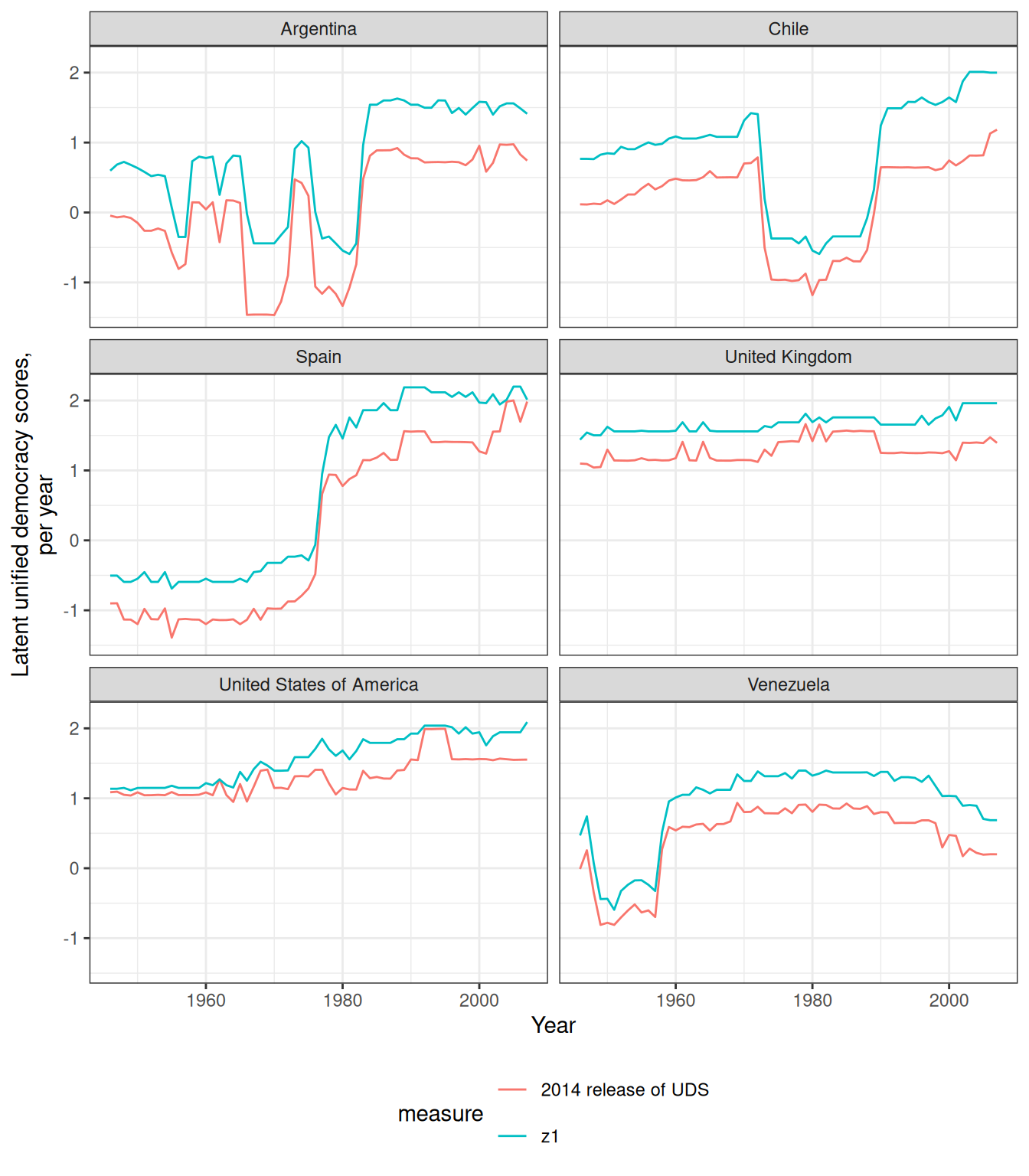
One important point to note about latent variable democracy scores is that they are normalized with mean zero and standard deviation one, so a score of 1 just means that the country-year is 1 standard deviation more democratic than the average country-year in the sample. But this means that adding extra country-years to our model will typically result in scores that have a higher mean (though usually smaller standard errors) than the original UD model, given that the world has become substantially more democratic over the last two centuries:

countries <- c("United States of America", 
               "United Kingdom","Argentina",
               "Chile","Venezuela","Spain")

data <- extended_scores %>% 
  filter(extended_country_name %in% countries) %>%
  tidyr::gather(measure, zscore, uds_2010_mean:uds_2014_mean, z1) %>%
  filter(!is.na(zscore), year >=1946, year < 2008) %>%
  mutate(measure = plyr::mapvalues(measure, 
                                   c("uds_2010_mean",
                                     "uds_2011_mean",
                                     "uds_2014_mean",
                                     "z1_matched"),
                                   c("2010 release of UDS",
                                     "2011 release of UDS",
                                     "2014 release of UDS",
                                     "Extended replication score")))

## The following `from` values were not present in `x`: z1_matched

ggplot(data = data, 
       aes(x = year, y = zscore, color = measure)) + 
  geom_path() + 
  theme_bw() + 
  labs(x = "Year", y = "Latent unified democracy scores,\nper year")  + 
  theme(legend.position="bottom") + 
  guides(color = guide_legend(ncol = 1),fill = guide_legend(nrow = 1)) + 
  facet_wrap(~extended_country_name, ncol = 2)

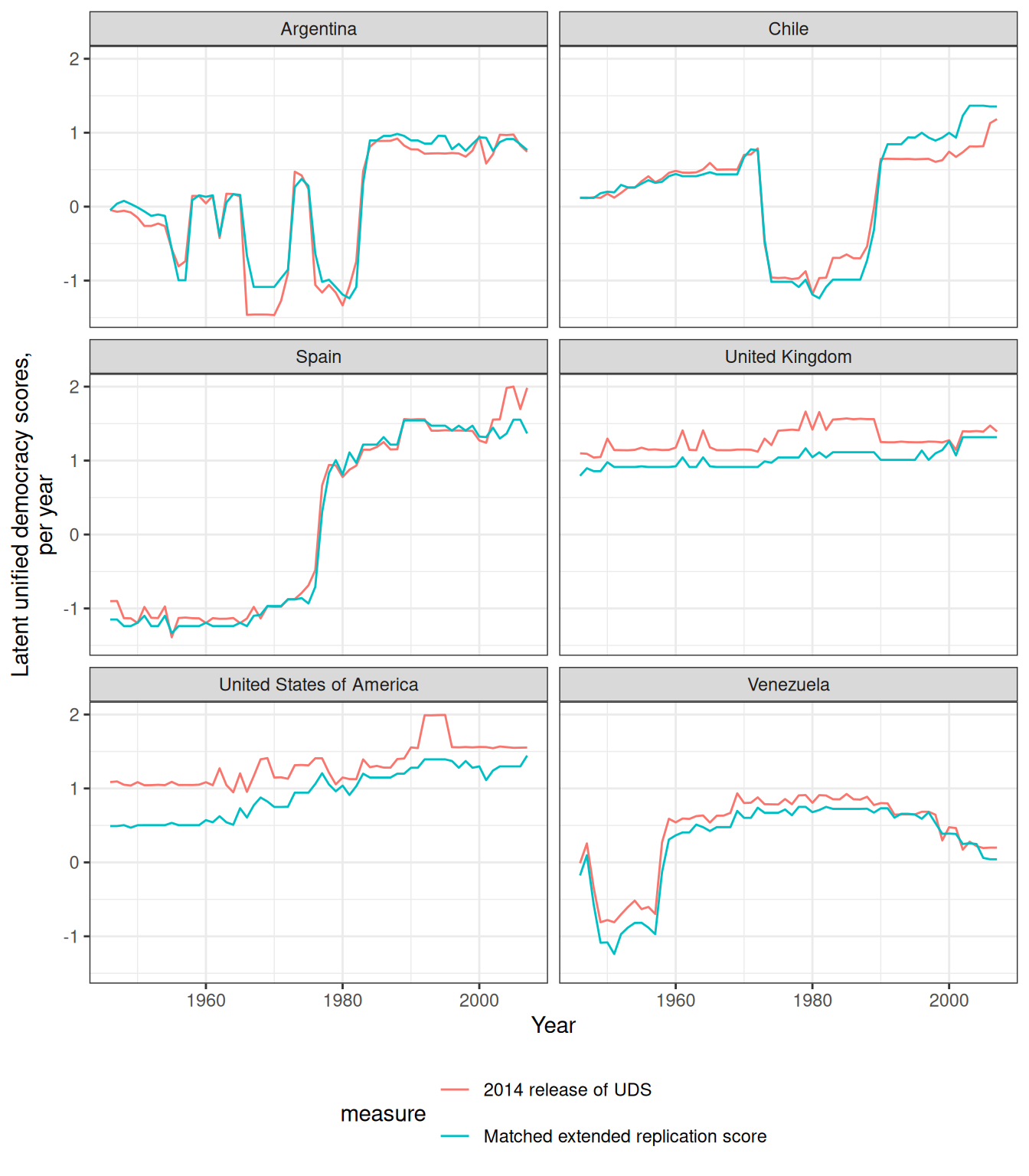
If necessary, one can therefore “match” the extended scores to the official UD release by substracting the mean of the extended scores for the period of the UD release one wants to match from the extended scores (that is, making the mean of the extended scores equal to zero for the period of adjustment):

matched_data <- extended_scores %>% 
  filter(!is.na(uds_2014_mean)) %>%
  mutate(z1_matched = z1 - mean(z1, na.rm = TRUE), 
         z1_pct975_matched = z1_pct975 - mean(z1, na.rm = TRUE), 
         z1_pct025_matched = z1_pct025 - mean(z1, na.rm = TRUE))

matched_data <- matched_data %>% 
  filter(extended_country_name %in% countries) %>%
  tidyr::gather(measure, zscore, uds_2010_mean:uds_2014_mean, z1_matched) %>%
  filter(!is.na(zscore), year >=1946, year < 2008) %>%
  mutate(measure = plyr::mapvalues(measure, 
                                   c("uds_2010_mean",
                                     "uds_2011_mean",
                                     "uds_2014_mean",
                                     "z1_matched"),
                                   c("2010 release of UDS",
                                     "2011 release of UDS",
                                     "2014 release of UDS",
                                     "Matched extended replication score")))

ggplot(data = matched_data, 
       aes(x = year, y = zscore, color = measure)) + 
  geom_path() + 
  theme_bw() + 
  labs(x = "Year", y = "Latent unified democracy scores,\nper year")  + 
  theme(legend.position="bottom") + 
  guides(color = guide_legend(ncol=1),fill = guide_legend(nrow=1)) + 
  facet_wrap(~extended_country_name,ncol=2)

In the graph above, we can see that the 2014 release of the UDS seems to overestimate the degree of democracy in the USA in the early decades of 1950 relative to the “extended” scores.

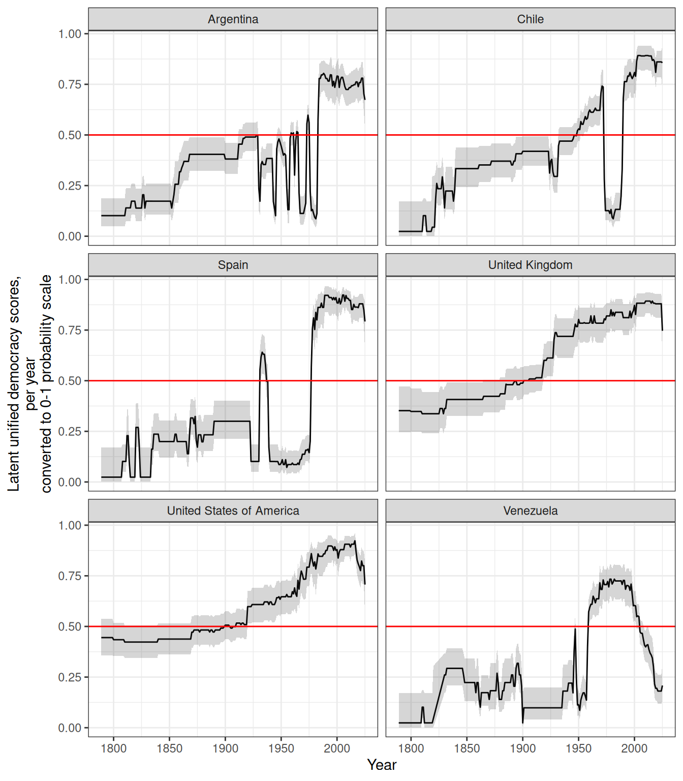
These scores have a more natural interpretation when transformed to a 0-1 index using the cumulative distribution function as the “probability that a country-year is democratic” (so the 0 is now a natural minimum, and 1 a natural maximum). These indexes are automatically produced by the function democracy_scores; they are in the column z1_as_prob of the output, and are produced by applying the pnorm function to z1, as follows:

extended_scores <- extended_scores %>% 
  mutate(index = pnorm(z1), 
         index_pct025 = pnorm(z1_pct025), 
         index_pct975 = pnorm(z1_pct975))

# These are equal to z1_as_prob, which is automatically calculated:

extended_scores %>% filter(index != z1_as_prob)

## # A tibble: 0 x 24
## # ... with 24 variables: extended_country_name <chr>, GWn <dbl>, cown <int>,
## #   in_GW_system <lgl>, year <dbl>, z1 <dbl>, se_z1 <dbl>, z1_pct975 <dbl>,
## #   z1_pct025 <dbl>, z1_adj <dbl>, z1_pct975_adj <dbl>, z1_pct025_adj <dbl>,
## #   z1_as_prob <dbl>, z1_pct975_as_prob <dbl>, z1_pct025_as_prob <dbl>,
## #   z1_adj_as_prob <dbl>, z1_pct975_adj_as_prob <dbl>,
## #   z1_pct025_adj_as_prob <dbl>, uds_2010_mean <dbl>, uds_2011_mean <dbl>,
## #   uds_2014_mean <dbl>, index <dbl>, index_pct025 <dbl>, ...

It is also possible to to set the cutpoint for this index at, for example, the average cutpoint in the latent variable of the dichotomous indexes of democracy (so that 0.5 correponds more naturally to the point at which a regime could be either democratic or non-democratic according to the dichotomous measures of democracy included in your model). These scores are also automatically calculated (they are in the column z1_adj) but they can also be manually added as follows:

cutpoints_extended <- cutpoints(extended_model)

cutpoints_extended

## # A tibble: 101 x 6
##    variable                     estimate pct025 pct975      se num_obs
##    <chr>                           <dbl>  <dbl>  <dbl>   <dbl>   <int>
##  1 pmm_arat                       -0.488 -0.493 -0.482 0.00290    3873
##  2 pmm_arat                       -0.157 -0.171 -0.143 0.00757    3873
##  3 pmm_arat                        0.275  0.240  0.314 0.0199     3873
##  4 pmm_arat                        0.564  0.507  0.626 0.0319     3873
##  5 pmm_arat                        0.951  0.862  1.05  0.0502     3873
##  6 pmm_arat                        1.74   1.58   1.91  0.0862     3873
##  7 blm                             0.519  0.331  0.813 0.150       505
##  8 blm                             1.11   0.715  1.74  0.318       505
##  9 bmr_democracy_femalesuffrage    0.888  0.787  1.00  0.0583    19129
## 10 pmm_bollen                     -0.620 -0.632 -0.605 0.00774     510
## # ... with 91 more rows

dichotomous_cutpoints <- cutpoints_extended %>% 
  group_by(variable) %>%
  filter(n() == 1) 

dichotomous_cutpoints

## # A tibble: 5 x 6
## # Groups:   variable [5]
##   variable                      estimate pct025 pct975     se num_obs
##   <chr>                            <dbl>  <dbl>  <dbl>  <dbl>   <int>
## 1 bmr_democracy_femalesuffrage     0.888  0.787  1.00  0.0583   19129
## 2 doorenspleet                     0.973  0.860  1.10  0.0654   13009
## 3 gwf_democracy_extended_strict    0.705  0.628  0.791 0.0440    9243
## 4 svolik_democracy                 0.763  0.674  0.863 0.0513    8555
## 5 ulfelder_democracy_extended      0.754  0.669  0.849 0.0486   11545

avg_dichotomous <- mean(dichotomous_cutpoints$estimate)

avg_dichotomous

## [1] 0.8165672

extended_scores <- extended_scores %>% mutate(adj_z1 = z1 - avg_dichotomous, 
                                        adj_pct025 = z1_pct025 - avg_dichotomous, 
                                        adj_pct975 =z1_pct975 - avg_dichotomous,
                                        index = pnorm(adj_z1),
                                        index_pct025 = pnorm(adj_pct025),
                                        index_pct975 = pnorm(adj_pct975))

ggplot(data = extended_scores %>% filter(extended_country_name %in% countries), 
       aes(x= year, y = index, 
           ymin = index_pct025, ymax = index_pct975)) + 
  geom_line() + 
  geom_ribbon(alpha=0.2) + 
  theme_bw() + 
  labs(x = "Year", y = "Latent unified democracy scores,\nper year\nconverted to 0-1 probability scale")  + 
  theme(legend.position="bottom") + 
  guides(color = guide_legend(ncol=1),fill = guide_legend(nrow=1)) + 
  geom_hline(yintercept=0.5,color="red") +
  facet_wrap(~extended_country_name,ncol=2)

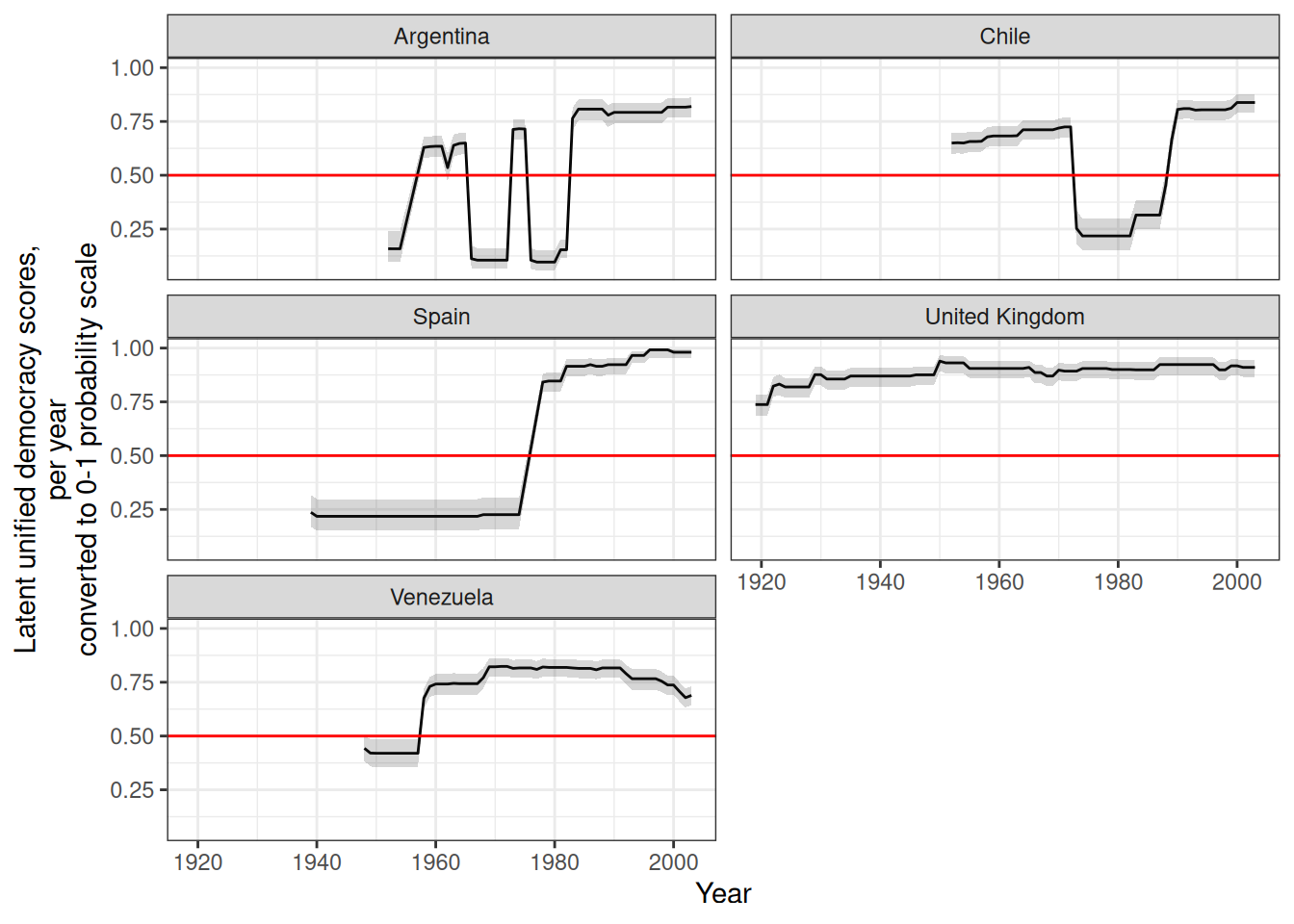
A pre-computed and documented version of the extended UDS scores, with data from all the indexes mentioned above, plus the participation-enhanced Polity Scores of Moon et al. (2006), a trichotomous democracy indicator calculated from Magaloni, Min, and Chu’s “Autocracies of the World” datset (Magaloni, Chu, and Min 2013), a dichotomous democracy indicator calculated from Hsu (2008), the REIGN dataset of Bell (2016), which extends Geddes, Wright, and Frantz (2014), a dichotomous democracy indicator from Acemoglu et al. (2019), the Bertelsmann Transformation index (Bertelsmann Stiftung 2022), and an indicator of democracy used by the Political Instability Task Force (Goldstone et al. 2010; Taylor and Ulfelder 2015), is included with the package; it can be loaded by simply typing extended_uds. Use ?extended_uds to examine the documentation for all its variables, and see my working paper (Marquez 2016) for more detail on the data and its uses.

The function generate_extended_uds() recreates these scores in one line of code, at the cost of some flexibility. It requires that the vdem package be installed; you can install it by using remotes::install_github("xmarquez/vdem).

Other Extensions

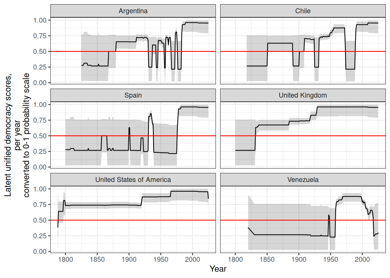
We can also use this method to create indexes from specific types of scores, such as dichotomous measures of democracy. Here we compute a 2-parameter logistic model from all dichotomous indexes of democracy (excluding near-duplicates):

dichotomous_dem <- all_dem %>%
  select(any_of(identifiers), where(~n_distinct(.) <= 3))  %>%
  select(-pacl, -pmm_pacl, -magaloni_democracy, 
         -bmr_democracy_omitteddata, -bmr_democracy, -bnr, 
         -wth_democ1, -ulfelder_democracy, 
         -gwf_democracy_extended, -utip_dichotomous)

dichotomous_dem <- prepare_democracy_data(dichotomous_dem)

dichotomous_model <- mirt(dichotomous_dem %>% select(-any_of(identifiers)),
                          model = 1, itemtype = "2PL", SE = TRUE, verbose = FALSE)

summary(dichotomous_model)

##                                  F1    h2
## anckar_democracy              0.995 0.990
## anrr_democracy                0.988 0.977
## bmr_democracy_femalesuffrage  0.992 0.984
## bnr_extended                  0.977 0.954
## doorenspleet                  0.978 0.957
## dsvmdi                        0.961 0.924
## fh_electoral                  0.984 0.968
## gwf_democracy_extended_strict 0.981 0.962
## kailitz_binary                0.981 0.963
## magaloni_democracy_extended   0.987 0.975
## pacl_update                   0.977 0.954
## PIPE_democracy                0.818 0.670
## pitf_binary                   0.977 0.955
## reign_democracy               0.975 0.951
## svolik_democracy              0.983 0.966
## ulfelder_democracy_extended   0.978 0.956
## utip_dichotomous_strict       0.949 0.900
## wth_democrobust               0.972 0.944
## 
## SS loadings:  16.95 
## Proportion Var:  0.942 
## 
## Factor correlations: 
## 
##    F1
## F1  1

dichotomous_scores <- democracy_scores(dichotomous_model)

dichotomous_scores <- bind_cols(dichotomous_dem %>% select(any_of(identifiers)),
                                dichotomous_scores)


ggplot(data = dichotomous_scores %>% filter(extended_country_name %in% countries), 
       aes(x= year, y = z1_as_prob, 
           ymin = z1_pct025_as_prob, ymax = z1_pct975_as_prob)) + 
  geom_line() + 
  geom_ribbon(alpha=0.2) + 
  theme_bw() + 
  labs(x = "Year", y = "Latent unified democracy scores,\nper year\nconverted to 0-1 probability scale")  + 
  theme(legend.position="bottom") + 
  guides(color = guide_legend(ncol=1),fill = guide_legend(nrow=1)) + 
  geom_hline(yintercept=0.5,color="red") +
  facet_wrap(~extended_country_name,ncol=2)

As Gründler and Krieger (2021) note, latent variable indexes suffer from arbitrary changes in level related to variables entering into or out of the source data. One way to get around this is to use a panel, with every measure present for every country-year in the panel. For example, suppose we’re interested only in measures with long coverage. Here we select a set of indexes with coverage down to the 19th century and then select the set of rows for which all measures exist, producing a panel with 159 countries and scores from 1919 to 2003.

full_panel <- all_dem %>%
  select(any_of(identifiers), reign_democracy, polity2, 
         bmr_democracy_femalesuffrage, v2x_polyarchy,
         ulfelder_democracy_extended, bnr_extended, 
         magaloni_democracy_extended, csvmdi, pitf,
         anckar_democracy, PEPS1v, vanhanen_democratization) %>%
  rowwise() %>%
  mutate(num_nas = sum(is.na(c_across(-any_of(identifiers))))) %>%
  filter(num_nas == 0) %>%
  ungroup() %>%
  select(-num_nas)

full_panel <- prepare_democracy_data(full_panel)

panel_model <- mirt(full_panel %>% select(-any_of(identifiers)),
                    model = 1, itemtype = "graded", SE = TRUE, 
                    verbose = FALSE, technical = list(NCYCLES = 1000))

panel_model@time

## TOTAL:   Data  Estep  Mstep     SE   Post 
##  14.06   0.08   0.81  12.50   0.66   0.00

summary(panel_model)

##                                 F1    h2
## reign_democracy              0.979 0.958
## polity2                      0.990 0.980
## bmr_democracy_femalesuffrage 0.984 0.968
## v2x_polyarchy                0.924 0.854
## ulfelder_democracy_extended  0.978 0.956
## bnr_extended                 0.975 0.951
## magaloni_democracy_extended  0.989 0.979
## csvmdi                       0.958 0.917
## pitf                         0.981 0.963
## anckar_democracy             0.986 0.972
## PEPS1v                       0.991 0.982
## vanhanen_democratization     0.948 0.898
## 
## SS loadings:  11.379 
## Proportion Var:  0.948 
## 
## Factor correlations: 
## 
##    F1
## F1  1

panel_scores <- democracy_scores(panel_model)

panel_scores <- bind_cols(full_panel %>% select(any_of(identifiers)),
                                panel_scores)

skimr::skim(panel_scores)

Data summary
Name	panel_scores
Number of rows	7102
Number of columns	18
_______________________
Column type frequency:
character	1
logical	1
numeric	16
________________________
Group variables	None

Variable type: character

skim_variable	n_missing	complete_rate	min	max	empty	n_unique	whitespace
extended_country_name	0	1	4	39	0	159	0

Variable type: logical

skim_variable	n_missing	complete_rate	mean	count
in_GW_system	0	1	1	TRU: 7102

Variable type: numeric

skim_variable	complete_rate	mean	sd	p0	p25	p50	p75	p100	hist
GWn	1	454.47	245.67	20.00	230.00	451.00	663.00	950.00	▇▇▇▇▅
cown	1	454.46	245.68	20.00	230.00	451.00	663.00	950.00	▇▇▇▇▅
year	1	1976.24	18.25	1919.00	1964.00	1978.00	1992.00	2003.00	▁▂▆▇▇
z1	1	-0.03	0.97	-2.12	-0.75	-0.16	0.73	2.41	▃▇▆▆▂
se_z1	1	0.11	0.06	0.02	0.08	0.11	0.13	0.40	▆▇▁▁▁
z1_pct975	1	0.19	0.95	-1.38	-0.51	0.01	0.91	3.13	▇▇▇▃▁
z1_pct025	1	-0.25	1.00	-2.90	-0.99	-0.32	0.53	1.71	▁▃▇▇▅
z1_adj	1	-0.38	0.97	-2.47	-1.10	-0.51	0.38	2.06	▃▇▆▆▂
z1_pct975_adj	1	-0.16	0.95	-1.73	-0.86	-0.34	0.56	2.78	▇▇▇▃▁
z1_pct025_adj	1	-0.60	1.00	-3.25	-1.34	-0.67	0.18	1.35	▁▃▇▇▅
z1_as_prob	1	0.49	0.30	0.02	0.23	0.44	0.77	0.99	▆▇▃▆▆
z1_pct975_as_prob	1	0.54	0.28	0.08	0.31	0.50	0.82	1.00	▆▇▅▅▇
z1_pct025_as_prob	1	0.43	0.30	0.00	0.16	0.38	0.70	0.96	▇▃▂▅▅
z1_adj_as_prob	1	0.39	0.29	0.01	0.14	0.31	0.65	0.98	▇▃▂▃▃
z1_pct975_adj_as_prob	1	0.44	0.29	0.04	0.20	0.37	0.71	1.00	▇▅▂▃▃
z1_pct025_adj_as_prob	1	0.34	0.28	0.00	0.09	0.25	0.57	0.91	▇▃▂▃▂

ggplot(data = panel_scores %>% filter(extended_country_name %in% countries), 
       aes(x= year, y = z1_as_prob, 
           ymin = z1_pct025_as_prob, ymax = z1_pct975_as_prob)) + 
  geom_line() + 
  geom_ribbon(alpha=0.2) + 
  theme_bw() + 
  labs(x = "Year", y = "Latent unified democracy scores,\nper year\nconverted to 0-1 probability scale")  + 
  theme(legend.position="bottom") + 
  guides(color = guide_legend(ncol=1),fill = guide_legend(nrow=1)) + 
  geom_hline(yintercept=0.5,color="red") +
  facet_wrap(~extended_country_name,ncol=2)

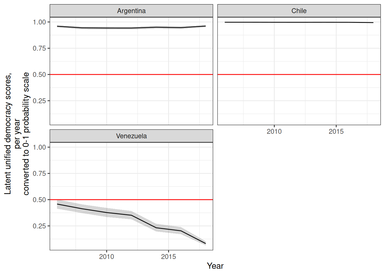
Or suppose we’re interested in a particular coverage period, including only measures that have data to 2018:

full_panel <- all_dem %>%
  pivot_longer(-any_of(identifiers), values_drop_na = TRUE) %>%
  filter(name %in% name[year == 2018]) %>%
  filter(year <= 2018) %>%
  pivot_wider(id_cols = any_of(identifiers), names_from = "name", values_from = "value") %>%
  unnest(fh_total_reversed:eiu) %>%
  select(-pitf_binary, -dsvmdi, -polityIV, -polity2IV, 
         -polity, -bti_democracy, -vanhanen_competition, 
         -vanhanen_participation) %>%
  rowwise() %>%
  mutate(num_nas = sum(is.na(c_across(-any_of(identifiers))))) %>%
  filter(num_nas == 0) %>%
  ungroup() %>%
  select(-num_nas)

full_panel <- prepare_democracy_data(full_panel)

panel_model <- mirt(full_panel %>% select(-any_of(identifiers)),
                    model = 1, itemtype = "graded", SE = TRUE, 
                    verbose = FALSE, technical = list(NCYCLES = 1000))

panel_model@time

## TOTAL:   Data  Estep  Mstep     SE   Post 
##  26.08   0.07   0.86  21.37   3.72   0.00

summary(panel_model)

##                                 F1    h2
## fh_total_reversed            0.938 0.879
## lexical_index                0.947 0.897
## lexical_index_plus           0.944 0.891
## v2x_api                      0.998 0.995
## v2x_libdem                   0.981 0.961
## v2x_mpi                      0.997 0.994
## v2x_partipdem                0.971 0.942
## v2x_polyarchy                0.998 0.997
## bmr_democracy                0.929 0.864
## bmr_democracy_femalesuffrage 0.929 0.864
## bmr_democracy_omitteddata    0.929 0.864
## pitf                         0.874 0.765
## polity2                      0.890 0.792
## v2x_delibdem                 0.966 0.934
## v2x_egaldem                  0.947 0.897
## csvmdi                       0.913 0.834
## vanhanen_democratization     0.717 0.514
## reign_democracy              0.851 0.724
## pacl_update                  0.865 0.748
## fh_electoral                 0.952 0.906
## wgi_democracy                0.943 0.889
## eiu                          0.889 0.790
## 
## SS loadings:  18.939 
## Proportion Var:  0.861 
## 
## Factor correlations: 
## 
##    F1
## F1  1

panel_scores <- democracy_scores(panel_model)

panel_scores <- bind_cols(full_panel %>% select(any_of(identifiers)),
                                panel_scores)

skimr::skim(panel_scores)

Data summary
Name	panel_scores
Number of rows	1722
Number of columns	18
_______________________
Column type frequency:
character	1
logical	1
numeric	16
________________________
Group variables	None

Variable type: character

skim_variable	n_missing	complete_rate	min	max	empty	n_unique	whitespace
extended_country_name	0	1	4	39	0	161	0

Variable type: logical

skim_variable	n_missing	complete_rate	mean	count
in_GW_system	0	1	1	TRU: 1722

Variable type: numeric

skim_variable	complete_rate	mean	sd	p0	p25	p50	p75	p100	hist
GWn	1	460.36	234.39	2.00	316.00	451.00	660.00	950.00	▅▇▇▇▃
cown	1	460.36	234.40	2.00	316.00	451.00	660.00	950.00	▅▇▇▇▃
year	1	2012.71	3.60	2006.00	2010.00	2013.00	2016.00	2018.00	▆▃▇▅▇
z1	1	0.11	1.30	-2.27	-1.00	0.00	1.09	3.01	▅▇▇▅▃
se_z1	1	0.05	0.04	0.00	0.01	0.03	0.08	0.24	▇▅▁▁▁
z1_pct975	1	0.20	1.33	-2.12	-0.91	0.03	1.22	3.49	▆▇▆▅▁
z1_pct025	1	0.02	1.27	-2.50	-1.07	-0.02	0.96	2.54	▅▇▇▆▆
z1_adj	1	0.44	1.30	-1.95	-0.67	0.33	1.42	3.34	▅▇▇▅▃
z1_pct975_adj	1	0.53	1.33	-1.79	-0.58	0.36	1.55	3.82	▆▇▆▅▁
z1_pct025_adj	1	0.35	1.27	-2.17	-0.75	0.31	1.29	2.86	▅▇▇▆▆
z1_as_prob	1	0.51	0.35	0.01	0.16	0.50	0.86	1.00	▇▃▅▃▇
z1_pct975_as_prob	1	0.53	0.34	0.02	0.18	0.51	0.89	1.00	▇▃▅▃▇
z1_pct025_as_prob	1	0.50	0.35	0.01	0.14	0.49	0.83	0.99	▇▃▃▃▇
z1_adj_as_prob	1	0.59	0.33	0.03	0.25	0.63	0.92	1.00	▅▃▂▃▇
z1_pct975_adj_as_prob	1	0.60	0.33	0.04	0.28	0.64	0.94	1.00	▅▂▂▃▇
z1_pct025_adj_as_prob	1	0.57	0.34	0.02	0.23	0.62	0.90	1.00	▅▃▂▃▇

ggplot(data = panel_scores %>% filter(extended_country_name %in% countries), 
       aes(x= year, y = z1_as_prob, 
           ymin = z1_pct025_as_prob, ymax = z1_pct975_as_prob)) + 
  geom_line() + 
  geom_ribbon(alpha=0.2) + 
  theme_bw() + 
  labs(x = "Year", y = "Latent unified democracy scores,\nper year\nconverted to 0-1 probability scale")  + 
  theme(legend.position="bottom") + 
  guides(color = guide_legend(ncol=1),fill = guide_legend(nrow=1)) + 
  geom_hline(yintercept=0.5,color="red") +
  facet_wrap(~extended_country_name,ncol=2)

Extracting useful information from a model

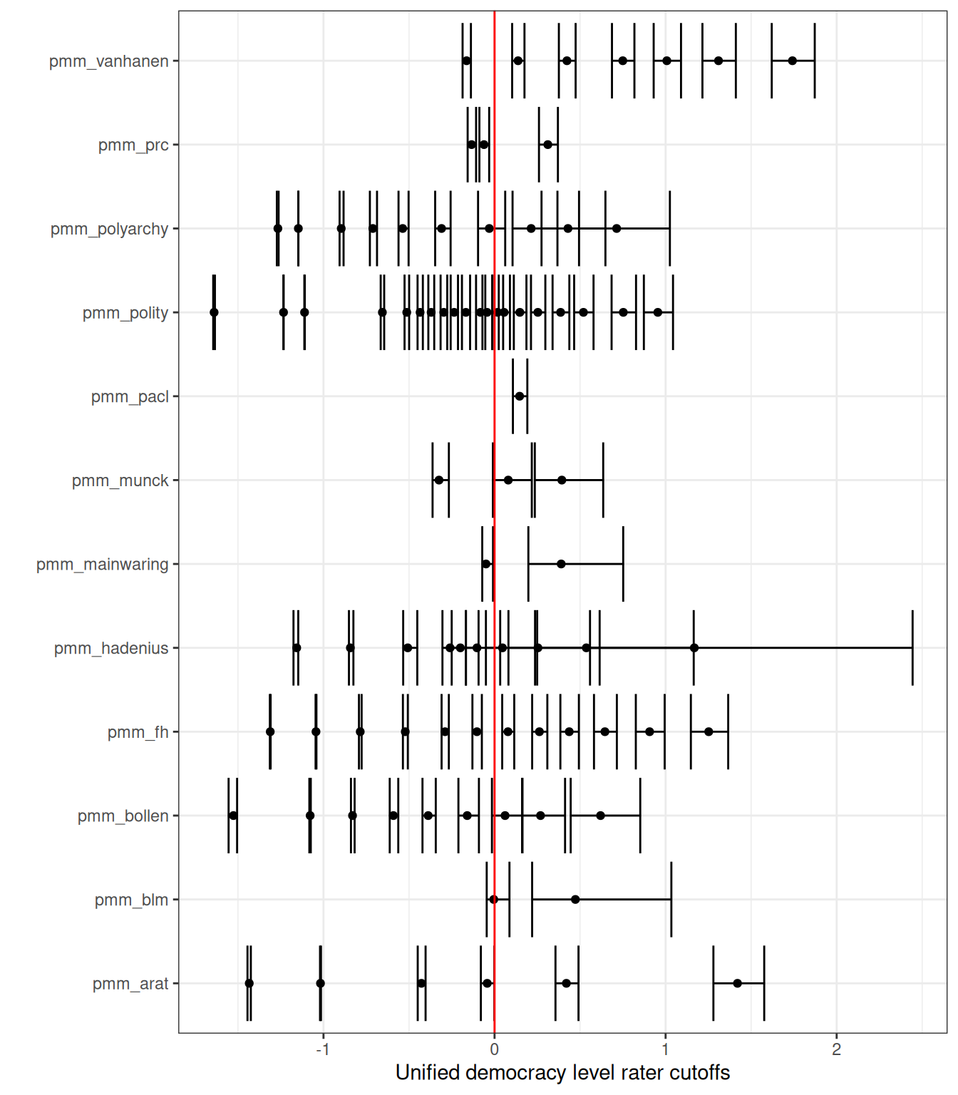
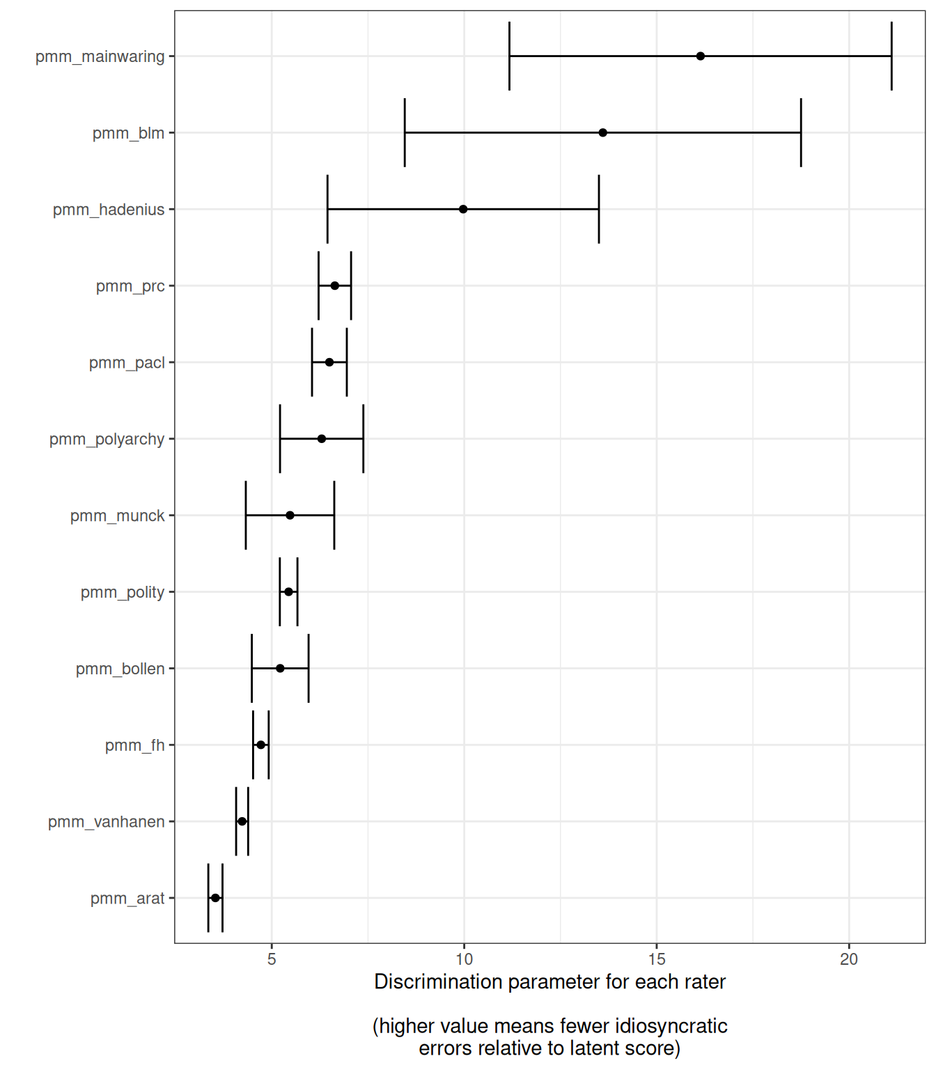
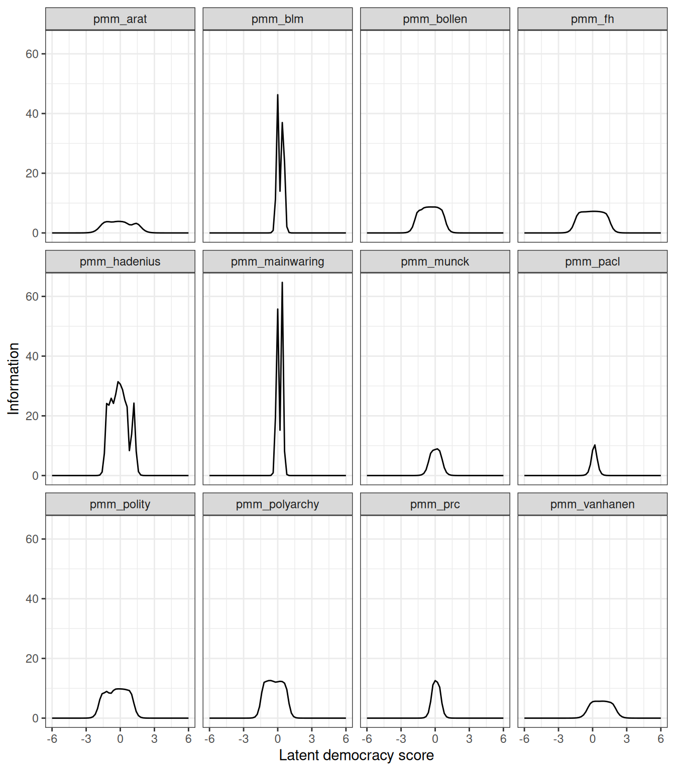
The mirt package offers a great number of powerful tools to examine and diagnose the fitted model, including functions to extract model cutpoints and item information curves. But this package also contains two convenience functions that wrap mirt tools to quickly extract democracy rater discrimination parameters, rater cutoffs, and rater information curves from a model produced by this procedure in a tidy data frame format suitable for graphing. Here, for example, we can replicate the figures in PMM’s original paper:

replication_2011_cutpoints <- cutpoints(replication_2011_model, type ="score")
replication_2011_cutpoints

## # A tibble: 85 x 6
##    variable   estimate  pct025    pct975      se num_obs
##    <chr>         <dbl>   <dbl>     <dbl>   <dbl>   <int>
##  1 pmm_arat   -1.43    -1.42   -1.44     0.00526    3873
##  2 pmm_arat   -1.02    -1.02   -1.01     0.00150    3873
##  3 pmm_arat   -0.427   -0.449  -0.403    0.0124     3873
##  4 pmm_arat   -0.0422  -0.0795 -0.000821 0.0211     3873
##  5 pmm_arat    0.421    0.357   0.491    0.0361     3873
##  6 pmm_arat    1.42     1.28    1.58     0.0798     3873
##  7 pmm_blm    -0.00364 -0.0451  0.0889   0.0472      275
##  8 pmm_blm     0.473    0.219   1.04     0.290       275
##  9 pmm_bollen -1.53    -1.50   -1.55     0.0145      510
## 10 pmm_bollen -1.08    -1.07   -1.08     0.00243     510
## # ... with 75 more rows

# We plot the "normalized" cutpoints ("estimate," in the same scale as the latent scores), 
# not the untransformed ones ("par")

ggplot(data = replication_2011_cutpoints, 
       aes(x = variable, y = estimate, 
           ymin = pct025, ymax = pct975))  + 
  theme_bw() + 
  labs(x="",y="Unified democracy level rater cutoffs") + 
  geom_point() + 
  geom_errorbar() + 
  geom_hline(yintercept =0, color="red") + 
  coord_flip()

# We can also plot discrimination parameters, which are in a different scale:
replication_2011_discrimination <- cutpoints(replication_2011_model, 
                                             type ="discrimination")

replication_2011_discrimination

## # A tibble: 12 x 5
##    variable       estimate pct025 pct975 num_obs
##    <chr>             <dbl>  <dbl>  <dbl>   <int>
##  1 pmm_arat           3.54   3.35   3.72    3873
##  2 pmm_blm           13.6    8.45  18.8      275
##  3 pmm_bollen         5.21   4.48   5.95     510
##  4 pmm_fh             4.72   4.51   4.92    6438
##  5 pmm_hadenius      10.1    6.48  13.7      129
##  6 pmm_mainwaring    16.2   11.2   21.2      835
##  7 pmm_munck          5.48   4.33   6.63     342
##  8 pmm_pacl           6.50   6.05   6.95    9067
##  9 pmm_polity         5.44   5.21   5.67    8050
## 10 pmm_polyarchy      6.29   5.21   7.37     353
## 11 pmm_prc            6.64   6.22   7.06    6002
## 12 pmm_vanhanen       4.23   4.07   4.39    8965

ggplot(data = replication_2011_discrimination, 
       aes(x=reorder(variable,estimate),
           y = estimate, ymin = pct025, 
           ymax = pct975))  + 
  theme_bw() + 
  labs(x="",y="Discrimination parameter for each rater
       \n(higher value means fewer idiosyncratic\nerrors relative to latent score)") + 
  geom_point() + 
  geom_errorbar() + 
  coord_flip()

# And we can plot item information curves for each rater:
replication_2011_info <- raterinfo(replication_2011_model)
replication_2011_info

## # A tibble: 732 x 3
##    rater    theta       info
##    <chr>    <dbl>      <dbl>
##  1 pmm_arat  -6   0.00000122
##  2 pmm_arat  -5.8 0.00000247
##  3 pmm_arat  -5.6 0.00000501
##  4 pmm_arat  -5.4 0.0000102 
##  5 pmm_arat  -5.2 0.0000206 
##  6 pmm_arat  -5   0.0000418 
##  7 pmm_arat  -4.8 0.0000847 
##  8 pmm_arat  -4.6 0.000172  
##  9 pmm_arat  -4.4 0.000349  
## 10 pmm_arat  -4.2 0.000707  
## # ... with 722 more rows

ggplot(data = replication_2011_info, aes(x=theta,y=info)) + 
  geom_path() + 
  facet_wrap(~rater) + 
  theme_bw() + 
  labs(x="Latent democracy score",y = "Information") + 
  theme(legend.position="bottom")

Finally, the package offers a simple function to estimate the probability that a given country is more democratic than another in a given year, accounting for the uncertainty in the UD-style measures. For example, suppose we want to know the probability that the USA was more democratic than France in the year 2000 for both the replicated 2011 scores and our extended model:

prob_more(replication_2011_scores, "United States of America","France", 2000)

## [1] 0.8781912

prob_more(extended_scores, "United States of America","France", 2000)

## [1] 0.7530363

Or perhaps we wish to know the probability that the United States was more democratic in the year 2000 than in the year 1953:

prob_more(replication_2011_scores, 
          "United States of America",
          "United States of America", 
          c(2000,1953))

## [1] 0.917908

prob_more(extended_scores, 
          "United States of America",
          "United States of America", 
          c(2000,1953))

## [1] 0.9999982

References

Acemoglu, Daron, Suresh Naidu, Pascual Restrepo, and James A. Robinson. 2019. “Democracy Does Cause Growth.” Journal of Political Economy 127 (1): 47–100. https://doi.org/10.1086/700936.

Anckar, Carsten, and Cecilia Fredriksson. 2018. “Classifying Political Regimes 1800-2016: A Typology and a New Dataset.” Journal Article. European Political Science. https://doi.org/10.1057/s41304-018-0149-8.

Arat, Zehra F. 1991. Democracy and Human Rights in Developing Countries. Boulder: Lynne Rienner Publishers.

Bell, Curtis. 2016. “The Rulers, Elections, and Irregular Governance Dataset (REIGN).” OEF Research. http://oefresearch.org/datasets/reign.

Bertelsmann Stiftung. 2022. “Transformation Index of the Bertelsmann Stiftung 2022.” Bertelsmann Stiftung.

Boix, Carles, Michael Miller, and Sebastian Rosato. 2012. “A Complete Dataset of Political Regimes, 1800-2007.” Comparative Political Studies 46 (12): 1523–54. https://doi.org/10.1177/0010414012463905.

Bollen, Kenneth A. 2001. “Cross-National Indicators of Liberal Democracy, 1950-1990.” Data set. Inter-university Consortium for Political; Social Research (ICPSR) [distributor].

Bowman, Kirk, Fabrice Lehoucq, and James Mahoney. 2005. “Measuring Political Democracy: Case Expertise, Data Adequacy, and Central America.” Comparative Political Studies 38 (8): 939–70. https://doi.org/10.1177/0010414005277083.

Chalmers, R. Philip. 2012. “Mirt: A Multidimensional Item Response Theory Package for the r Environment.” Journal Article. 2012 48 (6): 29. https://doi.org/10.18637/jss.v048.i06.

Cheibub, José, Jennifer Gandhi, and James Vreeland. 2010. “Democracy and Dictatorship Revisited.” Public Choice 143 (1): 67–101. https://doi.org/10.1007/s11127-009-9491-2.

Coppedge, Michael, Angel Alvarez, and Claudia Maldonado. 2008. “Two Persistent Dimensions of Democracy: Contestation and Inclusiveness.” The Journal of Politics 70 (03): 632–47. https://doi.org/10.1017/S0022381608080663.

Coppedge, Michael, John Gerring, Carl Henrik Knutsen, Staffan I. Lindberg, Jan Teorell, Nazifa Alizada, David Altman, et al. 2022. “V-Dem Country-Year/Country-Date Dataset v12.” Varieties of Democracy (V-Dem) Project. https://doi.org/10.23696/vdemds22.

Coppedge, Michael, and Wolfgang H. Reinicke. 1990. “Measuring Polyarchy.” Studies in Comparative International Development 25 (1): 51–72. https://doi.org/10.1007/Bf02716905.

Doorenspleet, Renske. 2000. “Reassessing the Three Waves of Democratization.” World Politics 52 (03): 384–406. https://doi.org/10.1017/S0043887100016580.

Freedom House. 2022. “Freedom in the World 2022: The Global Expansion of Authoritarian Rule.” Freedom House. https://freedomhouse.org/report/freedom-world/2022/global-expansion-authoritarian-rule.

Gasiorowski, Mark. 1996. “An Overview of the Political Regime Change Dataset.” Comparative Political Studies 29 (4): 469–83. https://doi.org/10.1177/0010414096029004004.

Geddes, Barbara, Joseph Wright, and Erica Frantz. 2014. “Autocratic Breakdown and Regime Transitions: A New Data Set.” Perspectives on Politics 12 (1): 313–31. https://doi.org/10.1017/S1537592714000851.

Goldstone, Jack, Robert Bates, David Epstein, Ted Gurr, Michael Lustik, Monty Marshall, Jay Ulfelder, and Mark Woodward. 2010. “A Global Model for Forecasting Political Instability.” American Journal of Political Science 54 (1): 190–208. https://doi.org/10.1111/j.1540-5907.2009.00426.x.

Gründler, Klaus, and Tommy Krieger. 2016. “Democracy and Growth: Evidence from a Machine Learning Indicator.” Journal Article. European Journal of Political Economy 45: 85–107. https://doi.org/https://doi.org/10.1016/j.ejpoleco.2016.05.005.

———. 2018. “Machine Learning Indices, Political Institutions, and Economic Development.” Report. CESifo Group Munich. https://www.cesifo-group.de/DocDL/cesifo1_wp6930.pdf.

———. 2021. “Using Machine Learning for Measuring Democracy: A Practitioners Guide and a New Updated Dataset for 186 Countries from 1919 to 2019.” European Journal of Political Economy, 102–47. https://doi.org/https://doi.org/10.1016/j.ejpoleco.2021.102047.

Hadenius, Axel. 1992. Democracy and Development. New York: Cambridge University Press.

Hsu, Sara. 2008. “The Effect of Political Regimes on Inequality, 1963-2002.” UTIP Working Paper, no. 53.

Kailitz, Steffen. 2013. “Classifying Political Regimes Revisited: Legitimation and Durability.” Democratization 20 (1): 39–60. https://doi.org/10.1080/13510347.2013.738861.

Kaufmann, Daniel, and Aart Kraay. 2020. “Worldwide Governance Indicators.” The World Bank Research Group. http://www.govindicators.org.

Magaloni, Beatriz, Jonathan Chu, and Eric Min. 2013. “Autocracies of the World, 1950-2012 (Version 1.0).” Dataset. http://cddrl.fsi.stanford.edu/research/autocracies_of_the_world_dataset.

Mainwaring, Scott, Aníbal Pérez-Liñán, and Daniel Brinks. 2014. “Political Regimes in Latin America, 1900-2007 (with Daniel Brinks).” In Democracies and Dictatorships in Latin America: Emergence, Survival, and Fall. New York: Cambridge University Press.

Marquez, Xavier. 2016. “A Quick Method for Extending the Unified Democracy Scores.” Journal Article. Available at SSRN 2753830. https://papers.ssrn.com/sol3/papers.cfm?abstract_id=2753830.

Marshall, Monty G., and Ted Robert Gurr. 2020. Polity 5: Political Regime Characteristics and Transitions, 1800-2018. Dataset Users’ Manual. Center for Systemic Peace.

Marshall, Monty G., Ted Robert Gurr, and Keith Jaggers. 2019. Polity IV Project: Political Regime Characteristics and Transitions, 1800-2018. Dataset Users’ Manual. Center for Systemic Peace.

Moon, Bruce E., Jennifer Harvey Birdsall, Sylvia Ciesluk, Lauren M. Garlett, Joshua J. Hermias, Elizabeth Mendenhall, Patrick D. Schmid, and Wai Hong Wong. 2006. “Voting Counts: Participation in the Measurement of Democracy.” Studies in Comparative International Development 41 (2): 3–32. https://doi.org/10.1007/BF02686309.

Munck, Gerardo. 2009. Measuring Democracy: A Bridge Between Scholarship and Politics. Baltimore: The Johns Hopkins University Press.

Pemstein, Daniel, Stephen A. Meserve, and James Melton. 2013. “Replication Data for: Democratic Compromise: A Latent Variable Analysis of Ten Measures of Regime Type.” Harvard Dataverse. http://hdl.handle.net/1902.1/PMM.

Pemstein, Daniel, Stephen Meserve, and James Melton. 2010. “Democratic Compromise: A Latent Variable Analysis of Ten Measures of Regime Type.” Political Analysis 18 (4): 426–49. https://doi.org/10.1093/pan/mpq020.

Przeworski, Adam. 2013. “Political Institutions and Political Events (PIPE) Data Set.” Data set. Department of Politics, New York University. https://sites.google.com/a/nyu.edu/adam-przeworski/home/data.

Reich, G. 2002. “Categorizing Political Regimes: New Data for Old Problems.” Democratization 9 (4): 1–24. https://doi.org/10.1080/714000289.

Skaaning, Svend-Erik, John Gerring, and Henrikas Bartusevičius. 2015. “A Lexical Index of Electoral Democracy.” Comparative Political Studies 48 (12): 1491–1525. https://doi.org/10.1177/0010414015581050.

Svolik, Milan. 2012. The Politics of Authoritarian Rule. Cambridge: Cambridge University Press.

Taylor, Sean J, and Jay Ulfelder. 2015. “A Measurement Error Model of Dichotomous Democracy Status.” Available at SSRN. https://doi.org/10.2139/ssrn.2726962.

The Economist Intelligence Unit. 2022. “Democracy Index 2021: The China Challenge.” The Economist Intelligence Unit.

Ulfelder, Jay. 2012. “Democracy/Autocracy Data Set.” Harvard Dataverse. http://hdl.handle.net/1902.1/18836.

Vanhanen, Tatu. 2019. “Measures of Democracy 1810-2018 [Dataset]. Version 8.0 (2019-06-17).” Tampere: Finnish Social Science Data Archive [distributor]. http://urn.fi/urn:nbn:fi:fsd:T-FSD1289.

Wahman, Michael, Jan Teorell, and Axel Hadenius. 2013. “Authoritarian Regime Types Revisited: Updated Data in Comparative Perspective.” Contemporary Politics 19 (1): 19–34. https://sites.google.com/site/authoritarianregimedataset/data.

For more detail on the models used to generate these indexes, and their characteristics, see my working paper (Marquez 2016), available at https://papers.ssrn.com/sol3/papers.cfm?abstract_id=2753830.↩︎

Xavier Marquez

2022-05-26

Preparing your democracy measures

Fitting a democracy model

Extending the model

Other Extensions

Extracting useful information from a model

References