Introduction

This vignette shows how to create and modify the index of personal power used in several chapters of my book Non-democratic Politics: Authoritarianism, Dictatorships, and Democratization (Palgrave Macmillan, 2016). It assumes that you have downloaded the replication package as follows:

if(!require(devtools)) {
  install.packages("devtools")
}

devtools::install_github('xmarquez/AuthoritarianismBook')

It also assumes you have the dplyr, ggplot2, scales, forcats, GGally, lubridate, reshape2, mirt, and knitr packages installed:

if(!require(dplyr)) {
  install.packages("dplyr")
}

if(!require(ggplot2)) {
  install.packages("ggplot2")
}

if(!require(scales)) {
  install.packages("forcats")
}

if(!require(forcats)) {
  install.packages("scales")
}

if(!require(GGally)) {
  install.packages("GGally")
}

if(!require(lubridate)) {
  install.packages("lubridate")
}

if(!require(reshape2)) {
  install.packages("reshape2")
}

if(!require(mirt)) {
  install.packages("mirt")
}

if(!require(knitr)) {
  install.packages("knitr")
}

Preparing the data

There are three types of measures of personalism that have been used by scholars. First, there are measures of legal or de-facto “constraints on the executive;” second, there are measures of how much of a regime is “taken up” by a single executive (e.g., tenure, executive turnover); and finally, there are “all things considered” qualitative judgments of whether a regime is a “personal” one. I use all three in constructing the index of personalism used in the book.

Indexes of constraints on the executive

The V-Dem dataset (Coppedge et al. 2016) contains three variables that measure constraints, legal or de facto, on the executive: an index of “legislative constraints on the executive” (v2xlg_legcon: “To what extent is the legislature and government agencies (e.g., comptroller general, general prosecutor, or ombudsman) capable of questioning, investigating, and exercising oversight over the executive?”), an index of “judicial constraints on the executive” (v2x_jucon: “To what extent does the executive respect the constitution and comply with court rulings, and to what extent is the judiciary able to act in an independent fashion?”), and an index of “executive corruption” (v2x_execorr: “How routinely do members of the executive, or their agents grant favors in exchange for bribes, kickbacks, or other material inducements, and how often do they steal, embezzle, or misappropriate public funds or other state resources for personal or family use?”). These are highly correlated, but we use all three, since they provide distinct information about the personalization of power in a regime:

library(AuthoritarianismBook)
library(dplyr)
library(reshape2)

personalism_data <- vdem %>% 
  select(country_name, GWn, year, in_system,
         v2xlg_legcon, v2x_jucon, v2x_execorr) %>%
  melt(id.vars = c("country_name", "GWn", "year", "in_system"), na.rm = TRUE)

And Polity IV has a measure of constraints on the executive, the exconst variable (excluding the transition/interruption/interregunum codes):

polity_annual <- polity_annual %>%  mutate(exconst = ifelse(unclass(exconst) < 4, NA, unclass(exconst) - 3))

personalism_data <- bind_rows(personalism_data, polity_annual %>%
                                select(country_name, GWn, year, exconst, in_system) %>%
                                melt(id.vars = c("country_name","GWn","year", "in_system"))) 

## Warning in bind_rows_(x, .id): Unequal factor levels: coercing to character

rm(polity_annual)

library(ggplot2)
library(GGally)
library(reshape2)

ggcorr(dcast(personalism_data, GWn + year + in_system ~ variable) %>% 
         select(-GWn, -in_system, -year), label = TRUE,
  label_round = 2)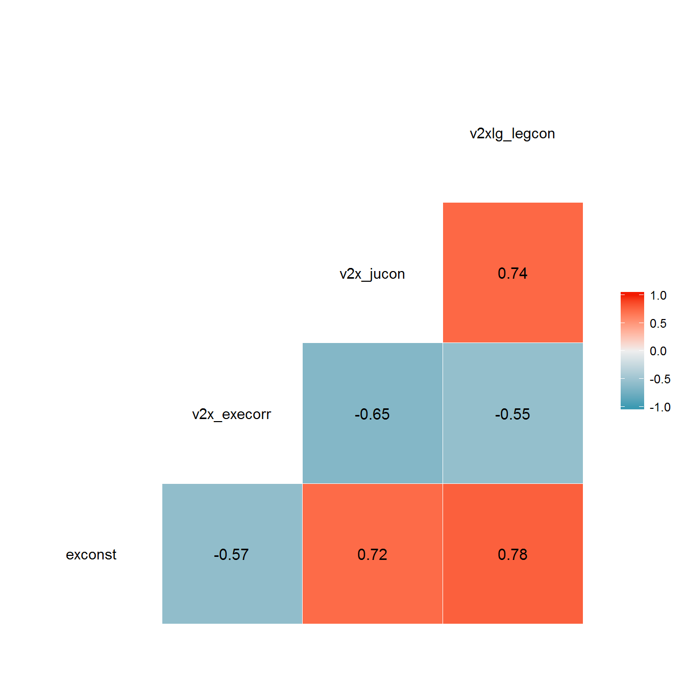

These measures are generally reasonable. Here’s the graph for Russia, for example:

library(lubridate)
library(purrr)
library(tidyr)

leader_data_yearly <- archigos %>%
  group_by(obsid, GWn, leader, startdate,enddate) %>%
  mutate(year = map2(startdate, enddate, ~ year(.x):year(.y))) %>%
  unnest() %>%
  group_by(GWn, year) %>%
  filter(enddate == max(enddate), startdate == max(startdate)) %>%
  group_by(leader) %>%
  mutate(is_start_leader_year = (year == min(year))) %>%
  ungroup()

country <- "Russia (Soviet Union)"
  
data <- left_join(personalism_data, leader_data_yearly) %>%
  filter(country_name %in% country)

## Joining, by = c("country_name", "GWn", "year")

extra_breaks <- NULL

extra_labels <- NULL

axis_labels <- data_frame(breaks = c(data$year[data$is_start_leader_year], extra_breaks),
                          labels = c(paste(data$year[data$is_start_leader_year],
                                    data$leader[data$is_start_leader_year]), extra_labels)) %>%
  distinct() %>%
  group_by(breaks) %>%
  summarise(labels = paste(labels, collapse = "\n"))


ggplot(data = data %>% 
         filter(grepl("v2", variable)), 
       aes(x=year, y = value,
           color = variable,
           fill = variable)) +
    geom_path() +
    facet_wrap(~country_name, ncol=2) +
    theme_bw() +
    scale_x_continuous(breaks = axis_labels$breaks,
                       labels = axis_labels$labels) +
    theme(axis.text.x = element_text(angle = 90, hjust = 1, vjust = 0.5)) +
    geom_vline(data = data %>%
                 filter(is_start_leader_year) %>%
                 distinct(leader,value, is_start_leader_year, .keep_all = TRUE),
               aes(xintercept = year)) +
    labs(y = "Degree of constraint/corruption
         (in standard deviations from mean, 
         0 is the mean in sample)", x = "Year") +
    theme(legend.position = "bottom") +
    guides(linetype = guide_legend(title = ""),
           color = guide_legend(title = ""),
           fill = guide_legend(title = ""))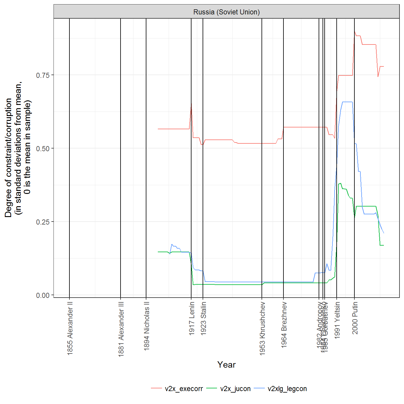

ggplot(data = data %>% 
         filter(grepl("exconst", variable)), 
       aes(x=year, y = value,
           color = variable,
           fill = variable)) +
    geom_path() +
    facet_wrap(~country_name, ncol=2) +
    theme_bw() +
    scale_x_continuous(breaks = axis_labels$breaks,
                       labels = axis_labels$labels) +
    theme(axis.text.x = element_text(angle = 90, hjust = 1, vjust = 0.5)) +
    geom_vline(data = data %>%
                 filter(is_start_leader_year) %>%
                 distinct(leader,value, is_start_leader_year, .keep_all = TRUE),
               aes(xintercept = year)) +
    labs(y = "Degree of constraint/corruption
         (in standard deviations from mean, 
         0 is the mean in sample)", x = "Year") +
    theme(legend.position = "bottom") +
    guides(linetype = guide_legend(title = ""),
           color = guide_legend(title = ""),
           fill = guide_legend(title = ""))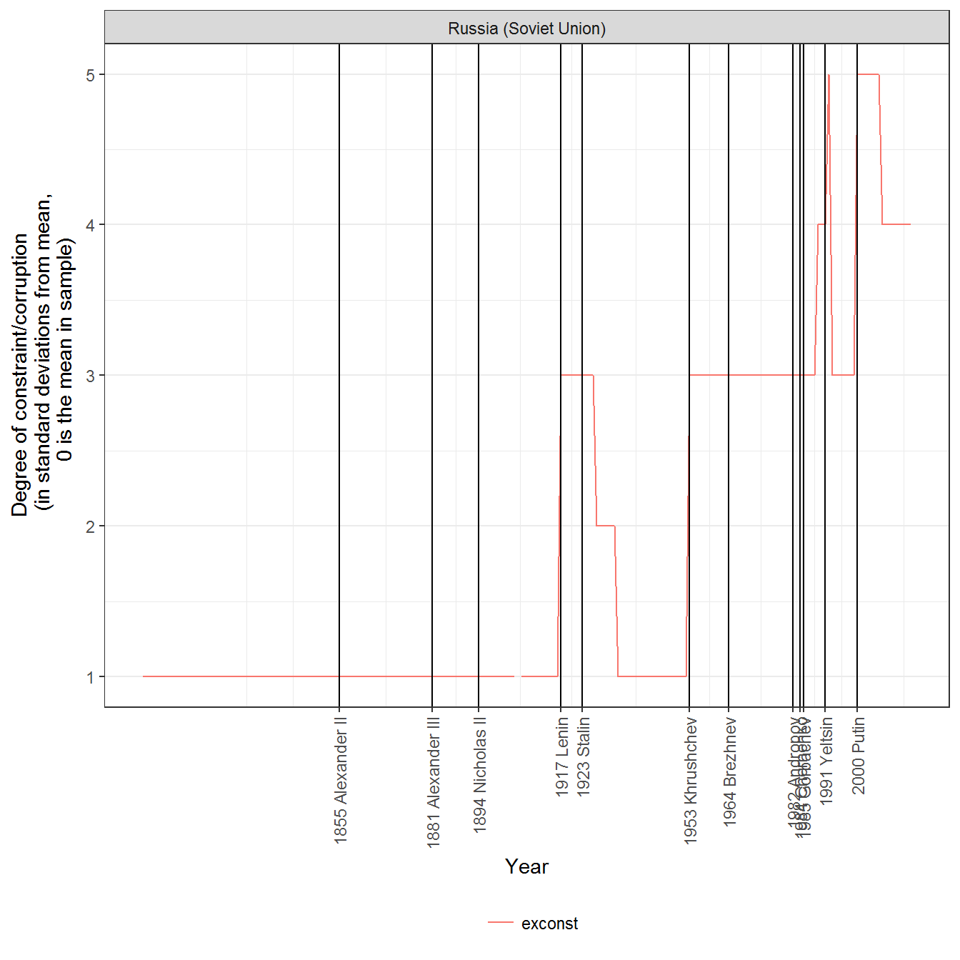

The graphs basically say that during Soviet times, legislative and executive constraints on the executive were greatly weakened. Executive corruption was at the mean in the sample, though it increased with Brezhnev (as we might have guessed from case knowledge), and it really shot upwards with the break up of the Soviet Union. At the same time, legislative and executive constraints increased until Putin came into office, when they began to decrease again.

Tenure-based measures of executive constraint

The dataset of regime types by Magaloni, Chu, and Min (2013) contains two measures of personalism: one derived from the exconst variable of the Polity IV dataset, and another one (lindex) which they describe as follows:

the variable is essentially a Herfindahl index (sum of squared shares) using the name of the executive. For a given country-year in a unique regime (see reg_id), the following calculation is made: \(\sum_{i=1}^m(exec_i/n)^2\) where n is the age of the regime up to that year, and exec is the number of years that a unique executive i (out of a total m executives up to that year) has led the regime. As such, a regime led by only one person up through that year yields a personalism index of 1. A theoretical scenario where leadership changes every single year would yield \(1/n\). These calculations are made using the non-rounded values. We note that this is a relatively sensitive measure in the early/formative years of an individual regime, but we propose this is a useful way of considering personalism as an evolving attribute of a regime over time.

I use this lindex variable only (since I directly included the exconst variable, noted above):

personalism_data <- bind_rows(personalism_data, magaloni %>%
                                select(country_name, GWn, year, in_system, lindex) %>%
                                melt(id.vars = c("country_name", "GWn", "year", "in_system"), na.rm = TRUE)) 

Wahman, Teorell, and Hadenius (Wahman, Teorell, and Hadenius 2013) also propose a measure of personalism based on “mean executive turnover”: the number of “changes of the chief executive during the regime spell, divided by the number of years of regime spell duration”, according" according to their regime classification. In a highly personalized regime this should be zero, while it ranges up to 3 chief executives per year for regimes with significant personnel turnover:

personalism_data <- bind_rows(personalism_data, wahman_teorell %>%
                                select(country_name, GWn, year, persagg1ny, in_system) %>%
                                melt(id.vars = c("country_name", "GWn", "year", "in_system"), na.rm= TRUE)) 

These measures are not well correlated with the measures of executive constraint or with one another. The lindex measure is also always 1 during the first year of the regime, which ensures it will always show “high” personalism at the time. This is perhaps justified as capturing the fact that new regimes are not yet highly institutionalized; every regime is highly personalized in its first year, until a regular transfer of power happens. But it is unintuitive, seemingly suggesting that both democratic and non-democratic regimes are equally personalized early on. At any rate, the lack of correlation between these measures indicates that they are at best measuring a different dimension of the phenomenon of personal rule than the constraints-based measures:

ggcorr(dcast(personalism_data, GWn + year + in_system ~ variable) %>% 
         select(-GWn:-in_system), label = TRUE,
  label_round = 2)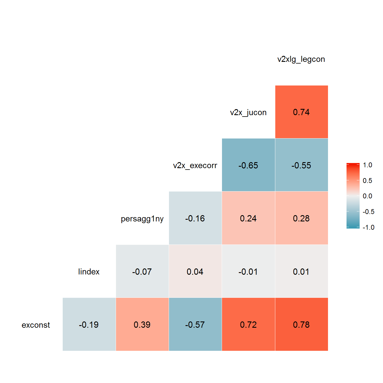

It is also worth noting that both lindex and persagg1ny are highly sensitive to the particular periodization of regimes used. For example, using Archigos (Goemans, Gleditsch, and Chiozza 2009), we can reconstruct both the Wahman, Teorell, and Hadenius (2013) and the Magaloni, Chu, and Min (2013) indexes for the Geddes, Wright, and Frantz (2014) classification of political regimes:

cumulative_levels <- function(seq) {
  seq <- as.factor(seq)
  levels(seq) <- seq_along(levels(seq))
  as.numeric(seq)
}

reconstruction <- magaloni %>%
  select(country_name, GWn, year, in_system, lindex) %>%
  full_join(magaloni_extended %>% 
              select(country_name, GWn, year, in_system, regime_nr)) %>%
  full_join(wahman_teorell %>% 
              select(country_name, GWn, year, in_system, regime1ny, persagg1ny)) %>%
  full_join(all_gwf_extended_yearly %>%
              select(country_name, GWn, year, in_system, gwf_casename, gwf_full_regimetype)) %>%
  full_join(leader_data_yearly) %>%
  arrange(country_name, year, startdate) %>%
  filter(!is.na(obsid), !is.na(gwf_casename)) %>%
  group_by(gwf_casename) %>%
  mutate(gwf_persagg1ny = (length(unique(obsid)) - 1)/length(unique(year))) %>%
  ungroup()

## Joining, by = c("country_name", "GWn", "year", "in_system")
## Joining, by = c("country_name", "GWn", "year", "in_system")
## Joining, by = c("country_name", "GWn", "year", "in_system")

## Joining, by = c("country_name", "GWn", "year")

ggcorr(reconstruction %>% 
         select(gwf_persagg1ny, persagg1ny, lindex), 
       label = TRUE,
       label_round = 2)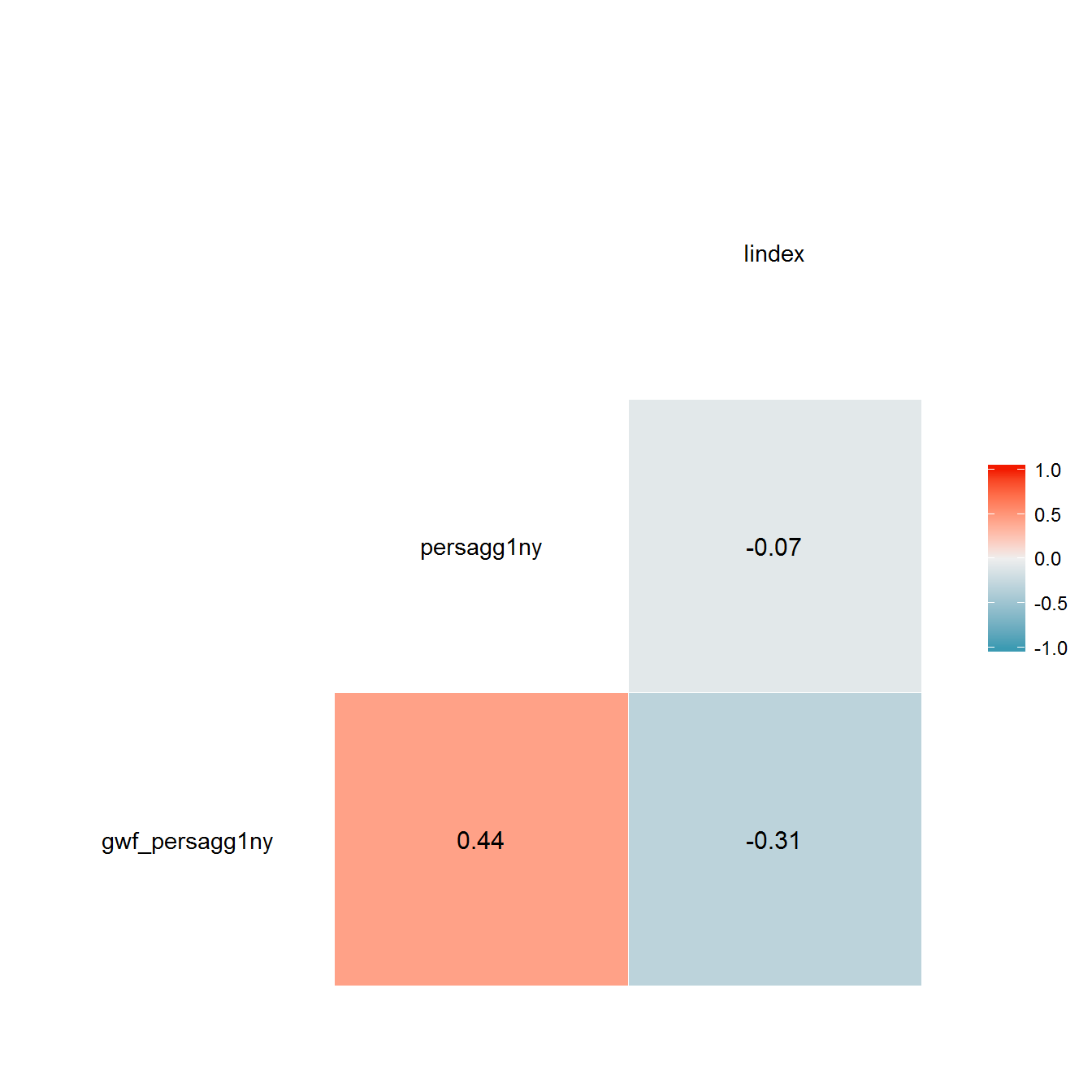

lindex_reconstruction <- reconstruction %>%
  group_by(gwf_casename) %>%
  arrange(year) %>%
  mutate(m = cumulative_levels(obsid),
         m = m - min(m) + 1,
         max_year = max(year)) %>%
  group_by(gwf_casename, obsid) %>%
  mutate(min_year = min(year),
         max_tenure = n()) %>%
  group_by(country_name, gwf_casename, leader, m, max_tenure, obsid) %>%
  do(data.frame(year = unique(.$min_year):unique(.$max_year))) %>%
  mutate(exec_i = seq_along(year),
         exec_i = ifelse(exec_i > max_tenure, 
                         max_tenure,
                         exec_i)) %>%
  group_by(gwf_casename) %>%
  arrange(year) %>%
  mutate(n = seq_along(year),
         share = (exec_i/n)^2) %>%
  group_by(country_name, gwf_casename, year) %>%
  summarise(gwf_lindex = sum(share))

reconstruction <- left_join(reconstruction, lindex_reconstruction)

## Joining, by = c("country_name", "year", "gwf_casename")

ggcorr(reconstruction %>% 
         select(gwf_persagg1ny, persagg1ny, lindex, gwf_lindex), 
       label = TRUE,
       label_round = 2)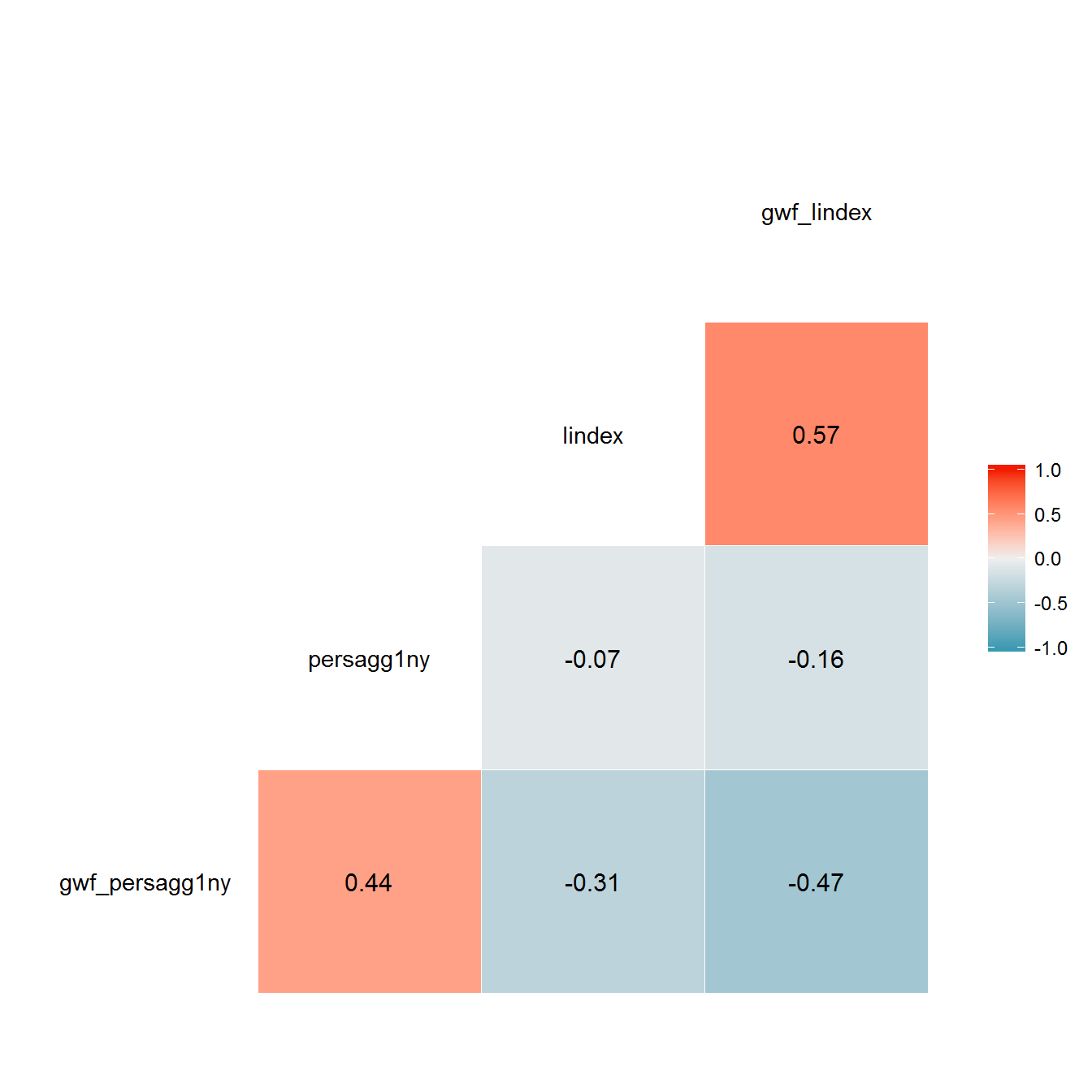

The correlations between the original and reconstructed variables are only moderately strong, since the regime periodizations in the respective datasets of political regimes are not identical. For example, here is what original and reconstructed variables look for Russia:

data <- reconstruction %>% 
  filter(country_name %in% country) %>%
  melt(measure.vars = c("gwf_persagg1ny", "persagg1ny", "lindex", "gwf_lindex"))

ggplot(data = data %>% filter(grepl("persa", variable)), 
       aes(x=year, y = value,
           color = variable,
           fill = variable)) +
    geom_path() +
    facet_wrap(~country_name, ncol=2) +
    theme_bw() +
    scale_x_continuous(breaks = axis_labels$breaks,
                       labels = axis_labels$labels) +
    theme(axis.text.x = element_text(angle = 90, hjust = 1, vjust = 0.5)) +
    geom_vline(data = data %>%
                 filter(is_start_leader_year) %>%
                 distinct(leader,value, is_start_leader_year, .keep_all = TRUE),
               aes(xintercept = year)) +
    labs(y = "Persagg1ny", x = "Year") +
    theme(legend.position = "bottom") +
    guides(linetype = guide_legend(title = ""),
           color = guide_legend(title = ""),
           fill = guide_legend(title = ""))

## Warning: Removed 55 rows containing missing values (geom_path).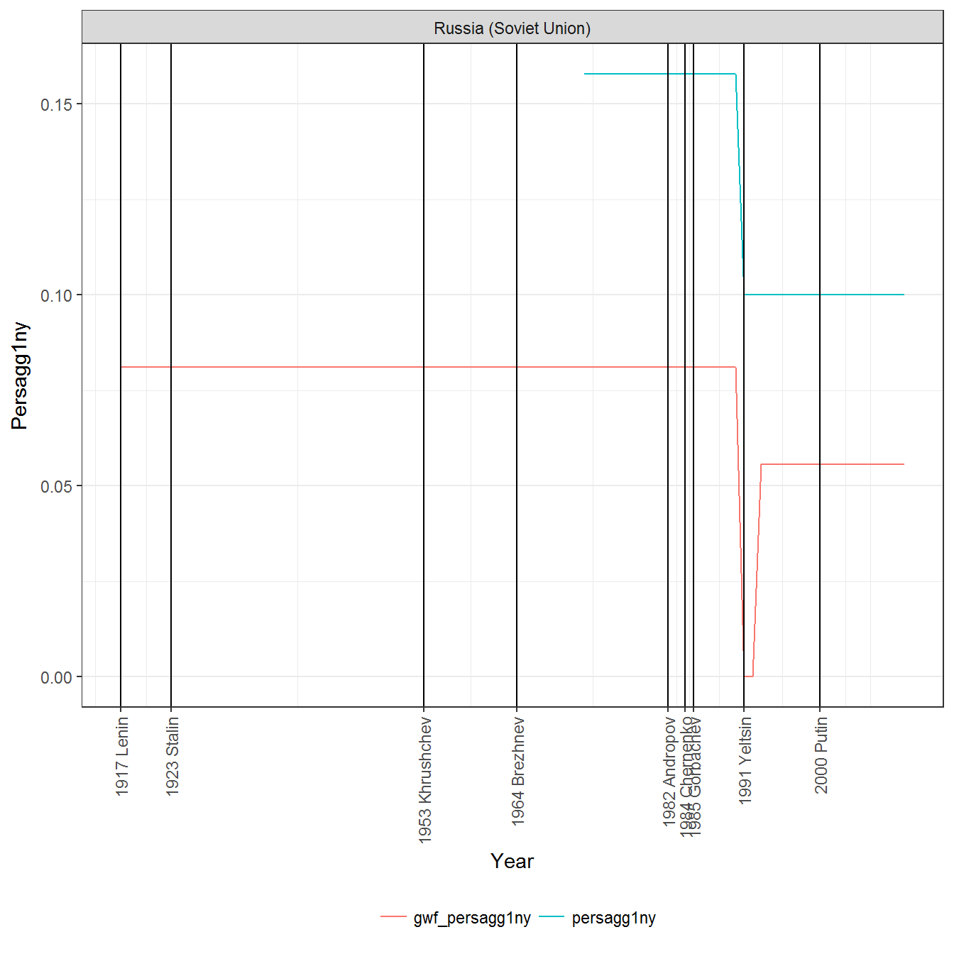

ggplot(data = data %>% filter(grepl("lindex", variable)), 
       aes(x=year, y = value,
           color = variable,
           fill = variable)) +
    geom_path() +
    facet_wrap(~country_name, ncol=2) +
    theme_bw() +
    scale_x_continuous(breaks = axis_labels$breaks,
                       labels = axis_labels$labels) +
    theme(axis.text.x = element_text(angle = 90, hjust = 1, vjust = 0.5)) +
    geom_vline(data = data %>%
                 filter(is_start_leader_year) %>%
                 distinct(leader,value, is_start_leader_year, .keep_all = TRUE),
               aes(xintercept = year)) +
    labs(y = "Lindex", x = "Year") +
    theme(legend.position = "bottom") +
    guides(linetype = guide_legend(title = ""),
           color = guide_legend(title = ""),
           fill = guide_legend(title = ""))

## Warning: Removed 33 rows containing missing values (geom_path).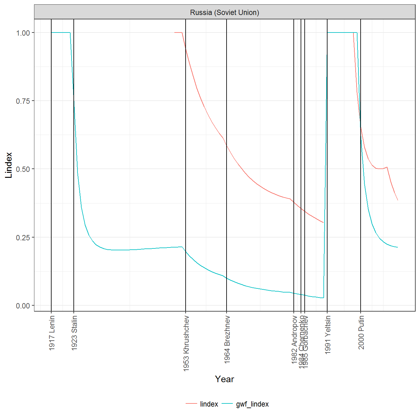

Because persagg1ny is invariant over the life of a regime, it is insensitive to fluctuations in personal power; by this measure, Lenin, Stalin, and Brezhnev all have the same amount of personal power over the life of the Soviet regime, since the “personalism” of the regime is averaged throughout its entire duration. Similarly, because lindex is always 1 at the beginning of a regime, the measure barely begins to capture Stalin’s personal power as his tenure lengthened. Despite these problems, we nevertheless include both lindex and persagg1ny in the construction of the personal power index; in any case the model will discount them when they are highly uncorrelated with the rest of the other measures.

personalism_data <- bind_rows(personalism_data, reconstruction %>%
                                select(country_name, GWn, year, in_system, gwf_lindex, gwf_persagg1ny) %>%
                                melt(id.vars = c("country_name","GWn","year", "in_system")))

personalism_data <- personalism_data %>% 
  filter(!is.na(value)) %>% 
  distinct()

ggcorr(dcast(personalism_data, country_name + GWn + year + in_system ~ variable) %>% 
         select(-country_name:-in_system), label = TRUE,
  label_round = 2)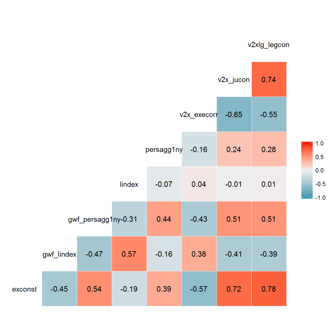

All-things-considered measures of personal rule

Finally, two datasets contain “all things considered” measures of whether a regime is “personal” (or has a personalistic component): Kailitz (2013) and Geddes, Wright, and Frantz (2014).

personalism_data <- bind_rows(personalism_data, kailitz_yearly %>%
                                select(country_name, GWn, year, in_system, personal) %>%
                                melt(id.vars = c("country_name", "GWn", "year", "in_system"))) 

all_gwf_extended_yearly <- all_gwf_extended_yearly %>%
  select(country_name, GWn, year, in_system, gwf_full_regimetype) %>%
  mutate(gwf_personal_single = grepl("^personal",gwf_full_regimetype),
         gwf_personal_hybrid  = grepl("personal",gwf_full_regimetype),
         gwf_personal = gwf_personal_single + gwf_personal_hybrid) %>%
  select(-gwf_personal_single,-gwf_personal_hybrid)

personalism_data <- bind_rows(personalism_data, all_gwf_extended_yearly %>%
                                select(-gwf_full_regimetype) %>%
                                melt(id.vars = c("country_name", "GWn", "year", "in_system"))) 

rm(all_gwf_extended_yearly)

Both of these measures represent coarse qualitative judgments, and are not perfectly correlated:

ggcorr(dcast(personalism_data, country_name + GWn + year + in_system ~ variable) %>% 
         select(gwf_personal, personal), label = TRUE,
  label_round = 2)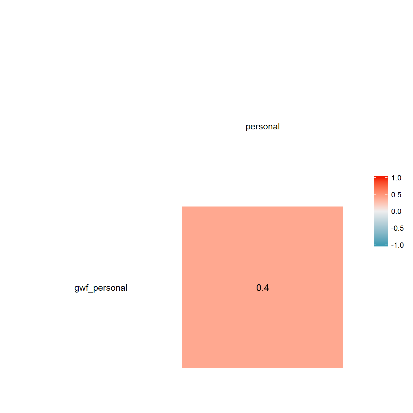

Nevertheless, both add some information to our index of personal power, and are therefore both used. The total correlation matrix looks like this:

ggcorr(data = dcast(personalism_data, GWn + year + in_system ~ variable) %>% 
         select(exconst:v2xlg_legcon),
       label = TRUE,
       label_round = 2)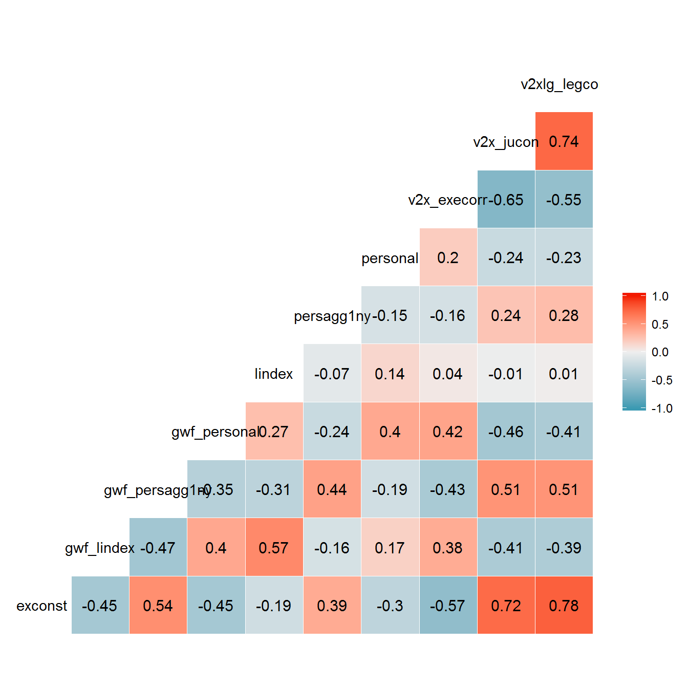

Creating the index

Cutting the data into a a manageable number of intervals

Before running the model, it is necessary to cut the continuous variables into a finite number of intervals. For entirely arbitrary reasons, I use 20 intervals. I also first transform the lindex and persagg1ny measures into percentile ranks. In the case of lindex, this smooths out some of the spikes of personal power at the beginning of a regime.

personalism_data <- dcast(personalism_data, country_name + GWn + year + in_system ~ variable)

summary(personalism_data)

##  country_name            GWn             year      in_system      
##  Length:22597       Min.   :  2.0   Min.   :1741   Mode :logical  
##  Class :character   1st Qu.:220.0   1st Qu.:1908   FALSE:5420     
##  Mode  :character   Median :432.0   Median :1949   TRUE :17177    
##                     Mean   :436.3   Mean   :1940   NA's :0        
##                     3rd Qu.:640.0   3rd Qu.:1985                  
##                     Max.   :990.0   Max.   :2015                  
##                                                                   
##     exconst        gwf_lindex    gwf_persagg1ny   gwf_personal  
##  Min.   :1.000   Min.   :0.000   Min.   :0.000   Min.   :0.000  
##  1st Qu.:1.000   1st Qu.:0.026   1st Qu.:0.036   1st Qu.:0.000  
##  Median :3.000   Median :0.217   Median :0.107   Median :0.000  
##  Mean   :3.777   Mean   :0.431   Mean   :0.149   Mean   :0.349  
##  3rd Qu.:7.000   3rd Qu.:1.000   3rd Qu.:0.220   3rd Qu.:0.000  
##  Max.   :7.000   Max.   :1.000   Max.   :0.985   Max.   :2.000  
##  NA's   :6310    NA's   :13286   NA's   :13286   NA's   :13030  
##      lindex        persagg1ny       personal      v2x_execorr   
##  Min.   :0.114   Min.   :0.000   Min.   :0.000   Min.   :0.011  
##  1st Qu.:0.515   1st Qu.:0.050   1st Qu.:0.000   1st Qu.:0.166  
##  Median :1.000   Median :0.125   Median :0.000   Median :0.440  
##  Mean   :0.762   Mean   :0.170   Mean   :0.062   Mean   :0.453  
##  3rd Qu.:1.000   3rd Qu.:0.250   3rd Qu.:0.000   3rd Qu.:0.726  
##  Max.   :1.000   Max.   :3.000   Max.   :1.000   Max.   :0.979  
##  NA's   :17444   NA's   :15904   NA's   :12991   NA's   :6268   
##    v2x_jucon      v2xlg_legcon  
##  Min.   :0.005   Min.   :0.023  
##  1st Qu.:0.267   1st Qu.:0.172  
##  Median :0.514   Median :0.450  
##  Mean   :0.517   Mean   :0.467  
##  3rd Qu.:0.777   3rd Qu.:0.754  
##  Max.   :0.992   Max.   :0.987  
##  NA's   :6268    NA's   :9309

personalism_data <- personalism_data %>% 
  mutate_at(.funs = funs(unclass(cut(., 
                               breaks = 20, 
                               include.lowest = TRUE, 
                               right = FALSE, 
                               ordered_result = TRUE))),
              .cols = c("v2x_execorr", "v2xlg_legcon", "v2x_jucon"))

personalism_data <- personalism_data %>% 
  mutate_at(.funs = funs(unclass(cut(percent_rank(.), 
                              20, 
                              include.lowest=TRUE, 
                              ordered_result=TRUE))),
              .cols = c("lindex", "gwf_lindex", "persagg1ny", "gwf_persagg1ny"))

personalism_data <- personalism_data %>% 
  mutate_at(.funs = funs(as.numeric(unclass(factor(., 
                                  ordered = TRUE)))), 
            .cols = c("v2x_execorr", "v2xlg_legcon", "v2x_jucon", "exconst",
                   "lindex", "gwf_lindex", "persagg1ny", "gwf_persagg1ny",
                   "personal", "gwf_personal"))

With these cuts, here is what the measures look like for Russia:

data <- left_join(personalism_data, leader_data_yearly) %>%
  filter(country_name %in% country) %>%
  melt(measure.vars = c("lindex",
                        "gwf_lindex",
                        "persagg1ny",
                        "gwf_persagg1ny",
                        "v2xlg_legcon", 
                        "v2x_jucon", 
                        "v2x_execorr",
                        "exconst"))

## Joining, by = c("country_name", "GWn", "year")

ggplot(data = data, 
       aes(x=year, y = value,
           color = variable,
           fill = variable)) +
    geom_path() +
    facet_wrap(~country_name, ncol=2) +
    theme_bw() +
    scale_x_continuous(breaks = axis_labels$breaks,
                       labels = axis_labels$labels) +
    theme(axis.text.x = element_text(angle = 90, hjust = 1, vjust = 0.5)) +
    geom_vline(data = data %>%
                 filter(is_start_leader_year) %>%
                 distinct(leader,value, is_start_leader_year, .keep_all = TRUE),
               aes(xintercept = year)) +
    labs(y = "Transformed variables", x = "Year") +
    theme(legend.position = "bottom") +
    guides(linetype = guide_legend(title = ""),
           color = guide_legend(title = ""),
           fill = guide_legend(title = ""))

## Warning: Removed 880 rows containing missing values (geom_path).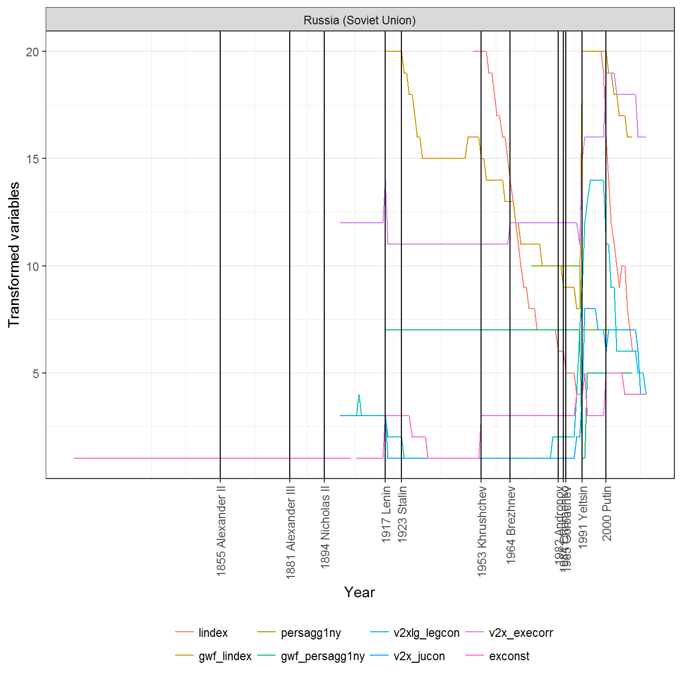

The correlations between the transformed variables are very similar to the correlations between the untransformed variables:

library(GGally)

ggcorr(data= personalism_data %>% select(exconst:v2xlg_legcon), label = TRUE, label_round = 2)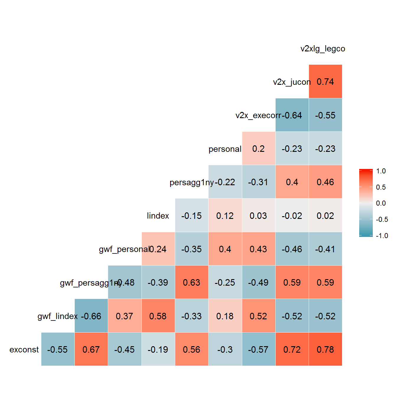

Running the model

Finally we create the model. Model 1 is the one used in the book:

data_1 <- personalism_data %>% 
  melt(measure.vars = c("exconst",
                        "gwf_personal",
                        "lindex", 
                        "persagg1ny",
                        "personal",
                        "v2x_execorr",
                        "v2x_jucon",
                        "v2xlg_legcon"),
       na.rm = TRUE) %>%
  dcast(country_name + GWn + year + in_system ~ variable)
  

library(mirt)
personal_model <- mirt(data_1 %>% 
                         select(exconst, 
                                gwf_personal,
                                lindex, 
                                persagg1ny,
                                personal,
                                v2x_execorr, 
                                v2x_jucon, 
                                v2xlg_legcon), 
                   model = 1, 
                   itemtype = "graded", 
                   SE = TRUE, 
                   verbose = FALSE)

personal_model

## 
## Call:
## mirt(data = data_1 %>% select(exconst, gwf_personal, lindex, 
##     persagg1ny, personal, v2x_execorr, v2x_jucon, v2xlg_legcon), 
##     model = 1, itemtype = "graded", SE = TRUE, verbose = FALSE)
## 
## Full-information item factor analysis with 1 factor(s).
## Converged within 1e-04 tolerance after 29 EM iterations.
## mirt version: 1.21 
## M-step optimizer: BFGS 
## EM acceleration: Ramsay
## Number of rectangular quadrature: 61
## 
## Information matrix estimated with method: crossprod
## Condition number of information matrix = 2575.065
## Second-order test: model is a possible local maximum
## 
## Log-likelihood = -182105.3
## Estimated parameters: 109 
## AIC = 364428.5; AICc = 364429.6
## BIC = 365303.3; SABIC = 364956.9

summary(personal_model)

##                  F1    h2
## exconst       0.848 0.719
## gwf_personal -0.743 0.552
## lindex       -0.266 0.071
## persagg1ny    0.442 0.196
## personal     -0.727 0.528
## v2x_execorr  -0.770 0.593
## v2x_jucon     0.912 0.832
## v2xlg_legcon  0.850 0.723
## 
## SS loadings:  4.214 
## Proportion Var:  0.527 
## 
## Factor correlations: 
## 
##    F1
## F1  1

In model 1, the latent factor is most closely correlated with the measures of executive constraint, though Kailitz and Geddes, Wright, and Frantz’s measures of personalism get some weight too.

Model 2 uses instead the constructed measures of lindex and persagg1ny created from GWF’s regime classification and the ARCHIGOS data:

data_2 <- personalism_data %>% 
  melt(measure.vars = c("exconst",
                        "gwf_personal",
                        "gwf_lindex", 
                        "gwf_persagg1ny",
                        "personal",
                        "v2x_execorr",
                        "v2x_jucon",
                        "v2xlg_legcon"),
       na.rm = TRUE) %>%
  dcast(country_name + GWn + year + in_system ~ variable)

personal_model_2 <- mirt(data_2 %>% 
                         select(v2x_execorr, v2xlg_legcon, v2x_jucon, exconst,
                   gwf_lindex, gwf_persagg1ny, personal, gwf_personal), 
                   model = 1, 
                   itemtype = "graded", 
                   SE = TRUE, 
                   verbose = FALSE)

personal_model_2

## 
## Call:
## mirt(data = data_2 %>% select(v2x_execorr, v2xlg_legcon, v2x_jucon, 
##     exconst, gwf_lindex, gwf_persagg1ny, personal, gwf_personal), 
##     model = 1, itemtype = "graded", SE = TRUE, verbose = FALSE)
## 
## Full-information item factor analysis with 1 factor(s).
## Converged within 1e-04 tolerance after 43 EM iterations.
## mirt version: 1.21 
## M-step optimizer: BFGS 
## EM acceleration: Ramsay
## Number of rectangular quadrature: 61
## 
## Information matrix estimated with method: crossprod
## Condition number of information matrix = 1897.445
## Second-order test: model is a possible local maximum
## 
## Log-likelihood = -199257.5
## Estimated parameters: 110 
## AIC = 398734.9; AICc = 398736
## BIC = 399617.7; SABIC = 399268.1

summary(personal_model_2)

##                    F1    h2
## v2x_execorr    -0.770 0.592
## v2xlg_legcon    0.840 0.705
## v2x_jucon       0.895 0.801
## exconst         0.855 0.731
## gwf_lindex     -0.641 0.411
## gwf_persagg1ny  0.631 0.398
## personal       -0.792 0.627
## gwf_personal   -0.818 0.668
## 
## SS loadings:  4.933 
## Proportion Var:  0.617 
## 
## Factor correlations: 
## 
##    F1
## F1  1

Model 2 puts a lot of weight on the GWF-based persagg1ny measure.

Model 3 excludes the tenure-based measures of personal power completely:

data_3 <- personalism_data %>% 
  melt(measure.vars = c("exconst",
                        "gwf_personal",
                        "personal",
                        "v2x_execorr",
                        "v2x_jucon",
                        "v2xlg_legcon"),
       na.rm = TRUE) %>%
  dcast(country_name + GWn + year + in_system ~ variable)

personal_model_3 <- mirt(data_3 %>% 
                         select(v2x_execorr, v2xlg_legcon, v2x_jucon, exconst,
                   personal, gwf_personal), 
                   model = 1, 
                   itemtype = "graded", 
                   SE = TRUE, 
                   verbose = FALSE)

personal_model_3

## 
## Call:
## mirt(data = data_3 %>% select(v2x_execorr, v2xlg_legcon, v2x_jucon, 
##     exconst, personal, gwf_personal), model = 1, itemtype = "graded", 
##     SE = TRUE, verbose = FALSE)
## 
## Full-information item factor analysis with 1 factor(s).
## Converged within 1e-04 tolerance after 184 EM iterations.
## mirt version: 1.21 
## M-step optimizer: BFGS 
## EM acceleration: Ramsay
## Number of rectangular quadrature: 61
## 
## Information matrix estimated with method: crossprod
## Condition number of information matrix = 2525.262
## Second-order test: model is a possible local maximum
## 
## Log-likelihood = -154163.4
## Estimated parameters: 72 
## AIC = 308470.9; AICc = 308471.3
## BIC = 309048.7; SABIC = 308819.9

summary(personal_model_3)

##                  F1    h2
## v2x_execorr  -0.774 0.599
## v2xlg_legcon  0.846 0.716
## v2x_jucon     0.920 0.847
## exconst       0.837 0.701
## personal     -0.710 0.504
## gwf_personal -0.733 0.537
## 
## SS loadings:  3.905 
## Proportion Var:  0.651 
## 
## Factor correlations: 
## 
##    F1
## F1  1

personal_scores <- fscores(personal_model, full.scores = TRUE, full.scores.SE = TRUE) %>% 
  data.frame() %>% 
  dplyr::rename(z1 = F1, se.z1 = SE_F1) %>% 
  mutate(pct975 = z1 + 1.96 * se.z1, pct025 = z1 - 1.96 * se.z1)

personal_scores <- bind_cols(data_1 %>% select(country_name, GWn, year), personal_scores)

personal_scores_2 <- fscores(personal_model_2, full.scores = TRUE, full.scores.SE = TRUE) %>% 
  data.frame() %>% 
  dplyr::rename(z1 = F1, se.z1 = SE_F1) %>% 
  mutate(pct975 = z1 + 1.96 * se.z1, pct025 = z1 - 1.96 * se.z1)

personal_scores_2 <- bind_cols(data_2 %>% select(country_name, GWn, year), personal_scores_2)

personal_scores_3 <- fscores(personal_model_3, full.scores = TRUE, full.scores.SE = TRUE) %>% 
  data.frame() %>% 
  dplyr::rename(z1 = F1, se.z1 = SE_F1) %>% 
  mutate(pct975 = z1 + 1.96 * se.z1, pct025 = z1 - 1.96 * se.z1)

personal_scores_3 <- bind_cols(data_3 %>% select(country_name, GWn, year), personal_scores_3)

personal_scores <- bind_rows(personal_scores, 
                             personal_scores_2, 
                             personal_scores_3, 
                             .id = "model")

rm(data_1, data_2, personal_scores_2, personal_scores_3)

The index right now is inverted - shows higher values of personal power as lower numbers - so we typically want to reverse it:

personal_scores <- personal_scores %>%
  mutate(z1 = -z1,
         pct975 = -pct975,
         pct025 = -pct025)

With that adjustment, this is what these scores look like for Russia:

data <- left_join(personal_scores, leader_data_yearly) %>%
  filter(country_name %in% country)

## Joining, by = c("country_name", "GWn", "year")

ggplot(data = data, 
       aes(x=year, y = z1,
           ymin = pct025,
           ymax = pct975,
           color = model,
           fill = model)) +
  geom_path() +
  geom_ribbon(alpha = 0.3) +
  facet_wrap(~country_name, ncol=2) +
  theme_bw() +
  scale_x_continuous(breaks = axis_labels$breaks,
                     labels = axis_labels$labels) +
  theme(axis.text.x = element_text(angle = 90, hjust = 1, vjust = 0.5)) +
  geom_vline(data = data %>%
               filter(is_start_leader_year) %>%
               distinct(leader, is_start_leader_year, .keep_all = TRUE),
             aes(xintercept = year)) +
  labs(y = "Index score", x = "Year") +
  theme(legend.position = "bottom") +
  guides(linetype = guide_legend(title = ""),
         color = guide_legend(title = "Model"),
         fill = guide_legend(title = "Model"))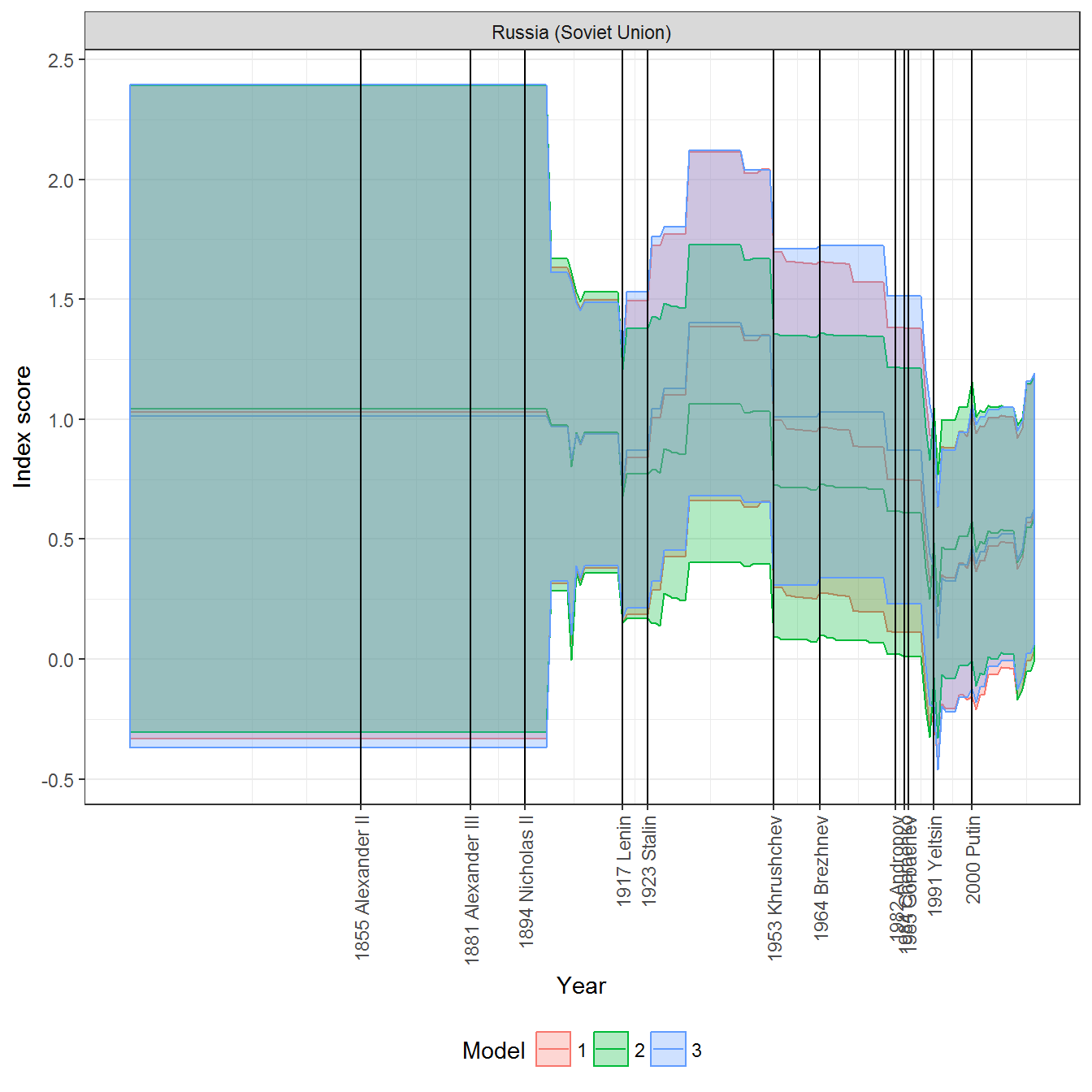

The scores from each of these models are in any case extremely well correlated:

data <- personal_scores %>%
  mutate(model = plyr::mapvalues(model, 
                                 from = c(1,2,3),
                                 to = c("Model_1_in_book","Model_2","Model_3"))) %>%
  dcast(country_name + GWn + year ~ model, value.var = "z1") %>%
  select(Model_1_in_book:Model_3)

ggcorr(data = data, label = TRUE, label_round = 2)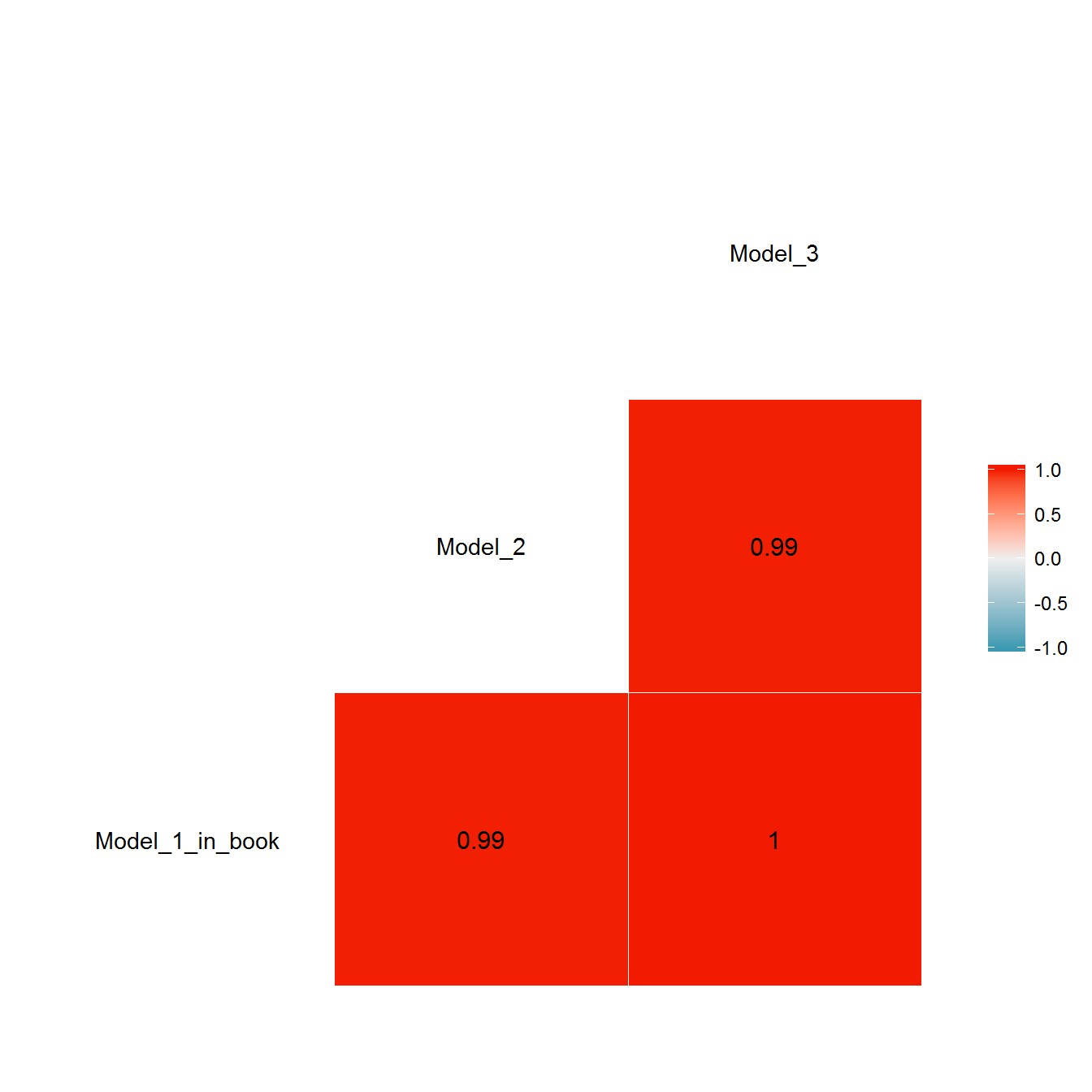

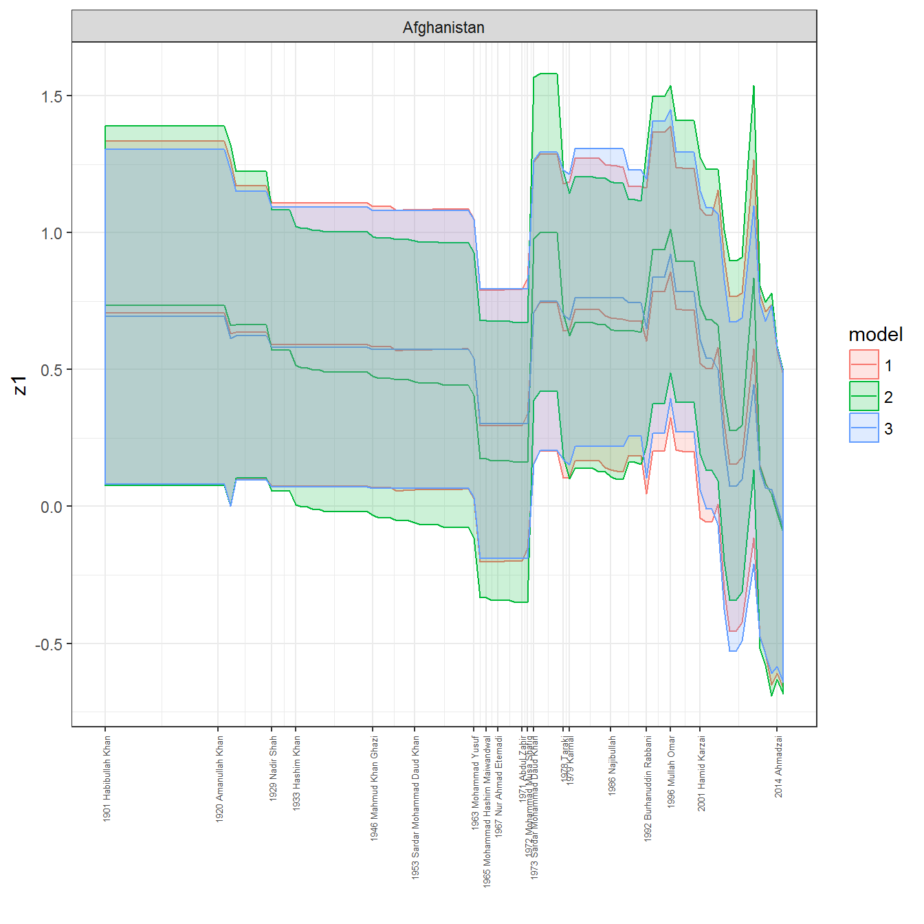
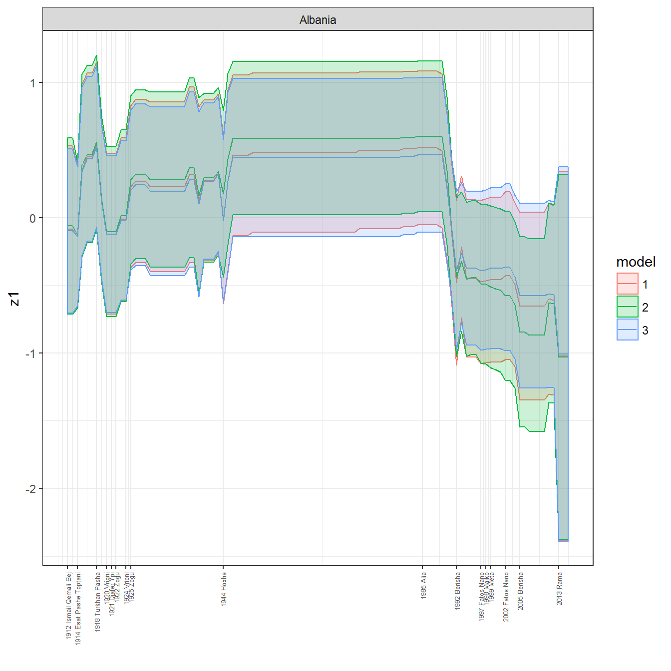
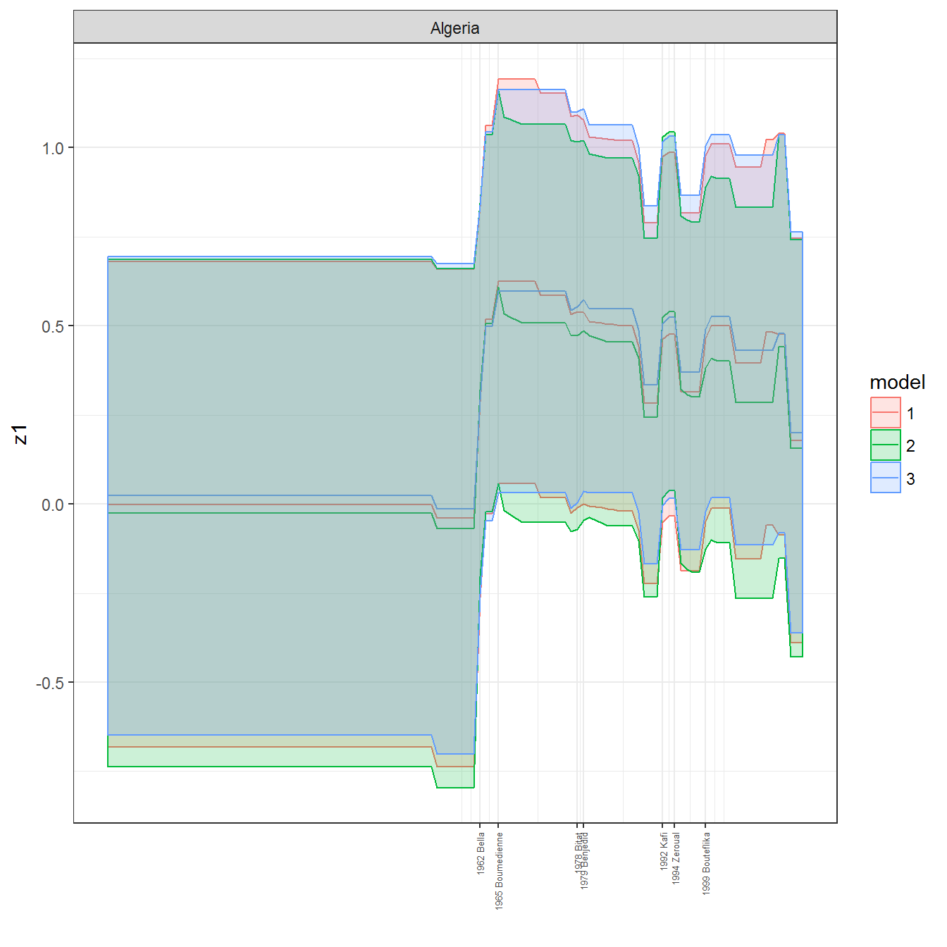
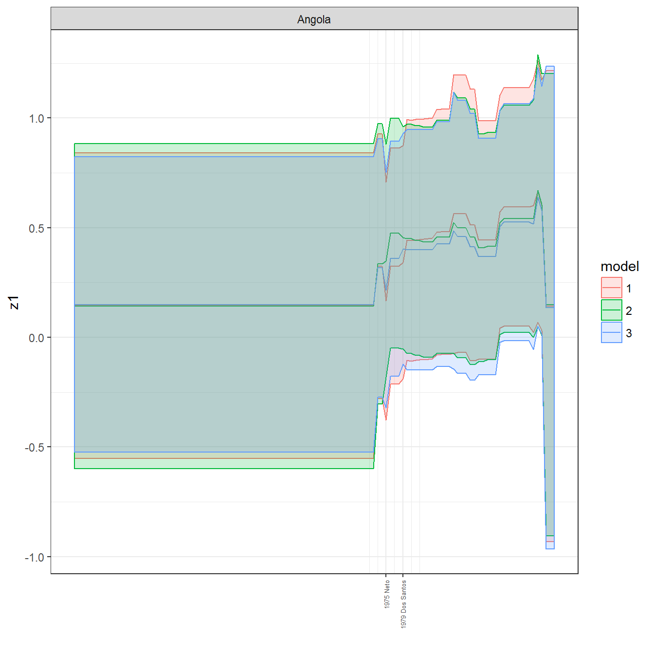
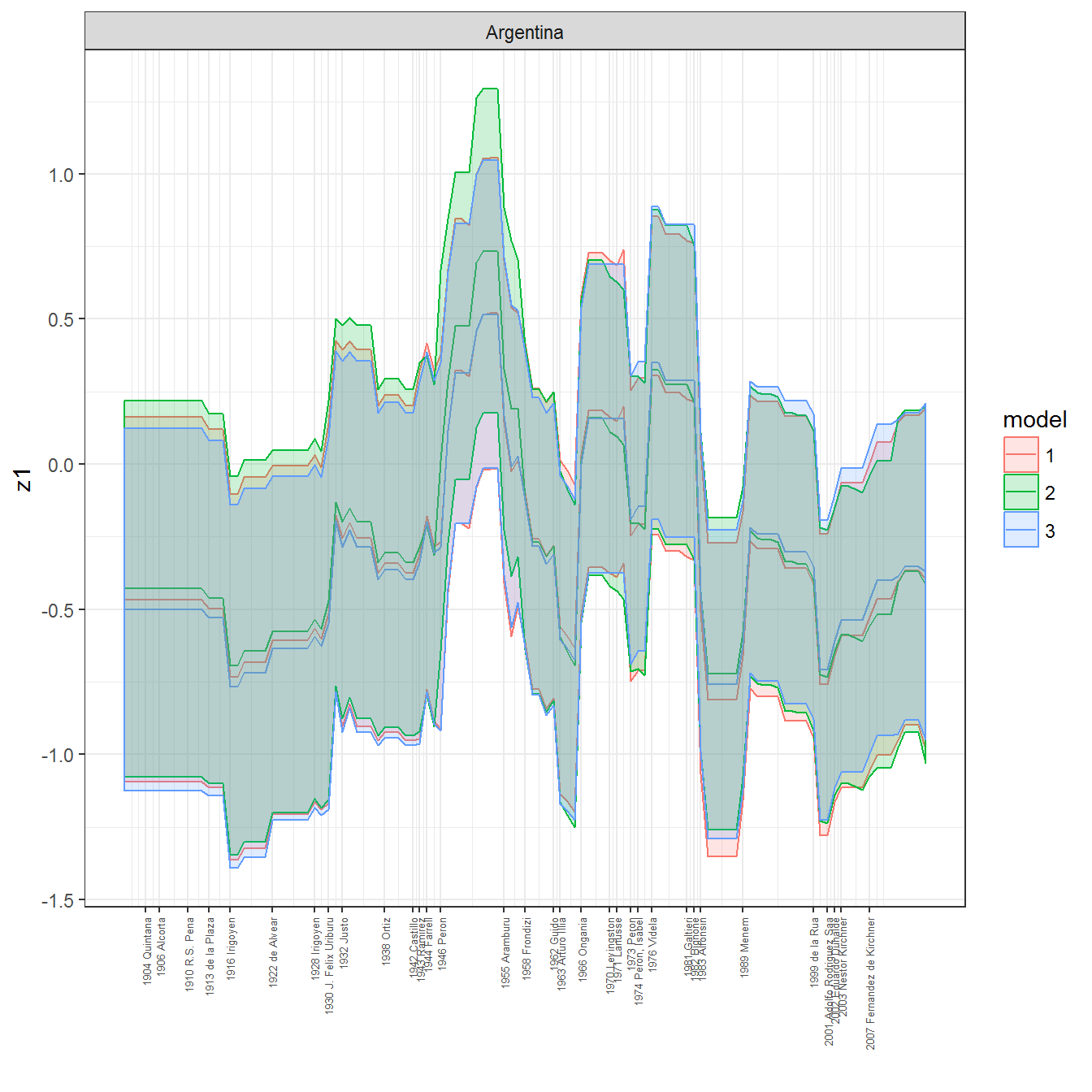
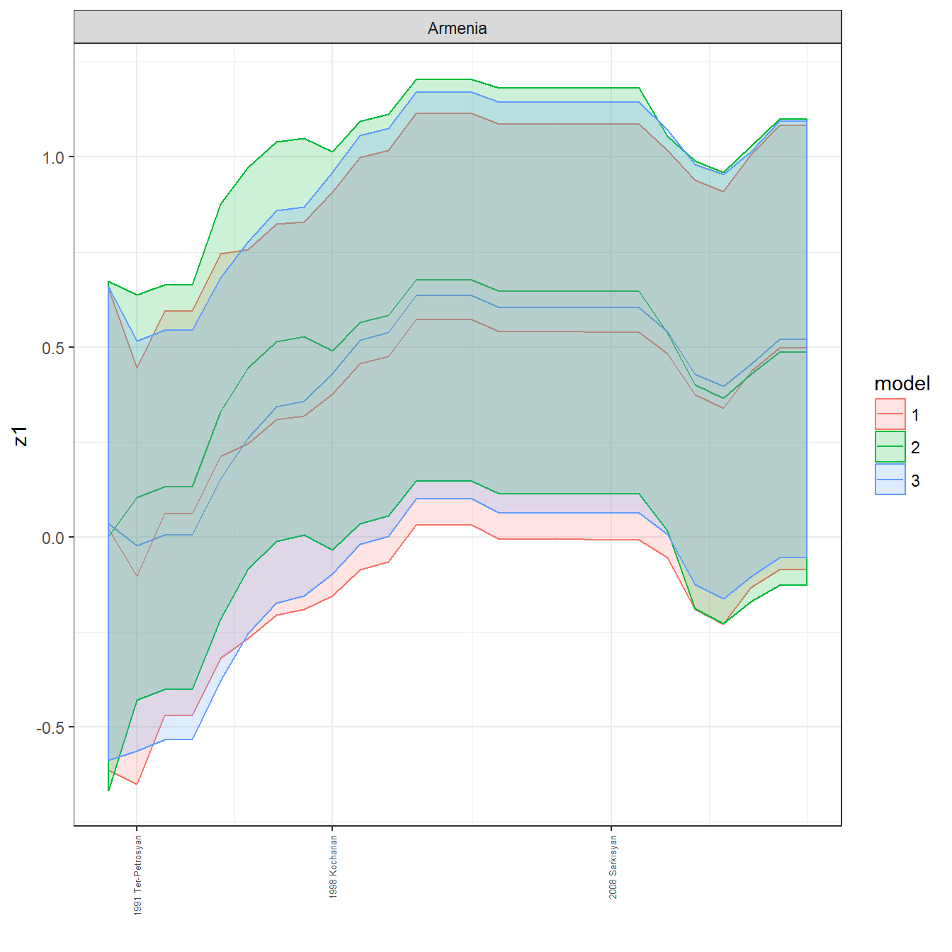
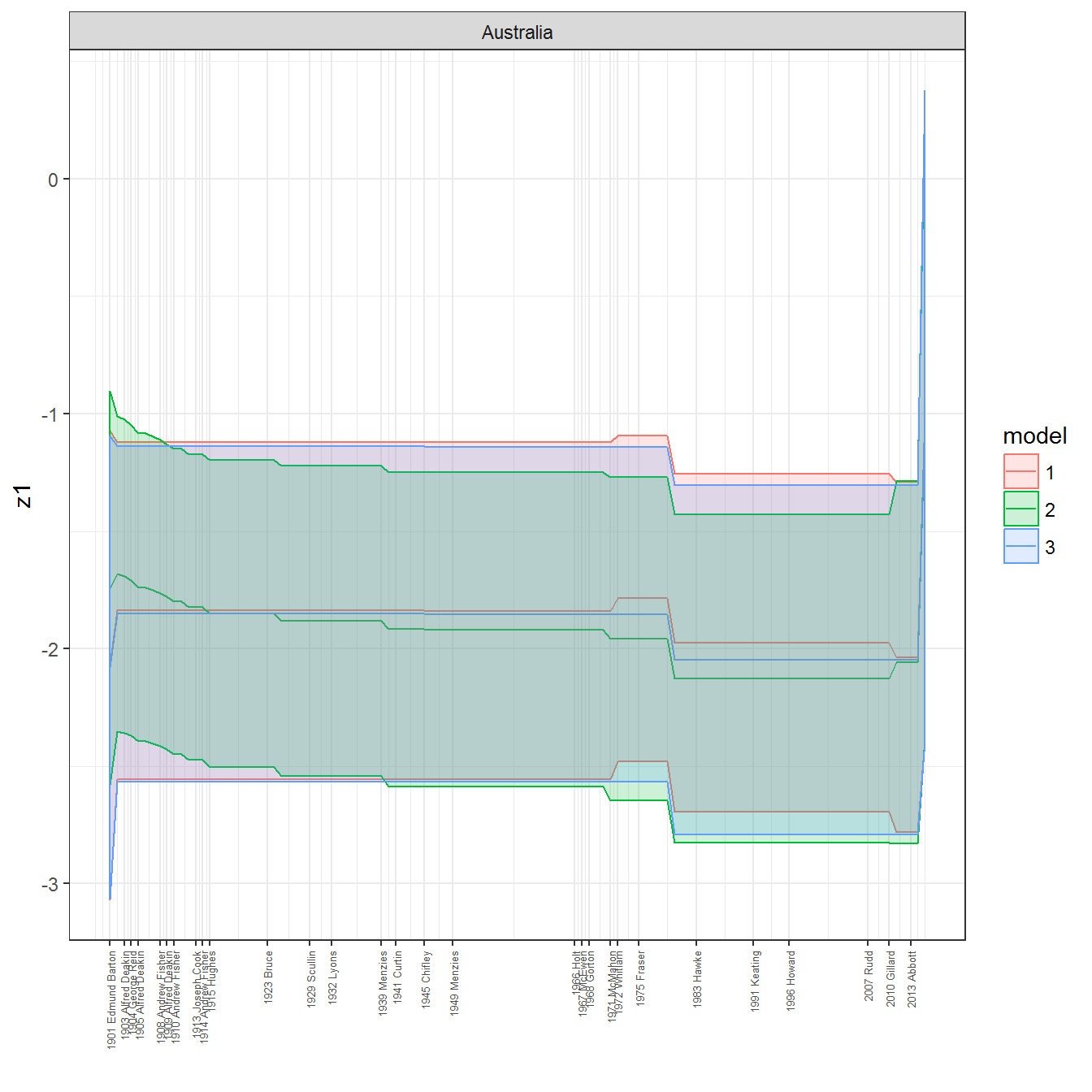
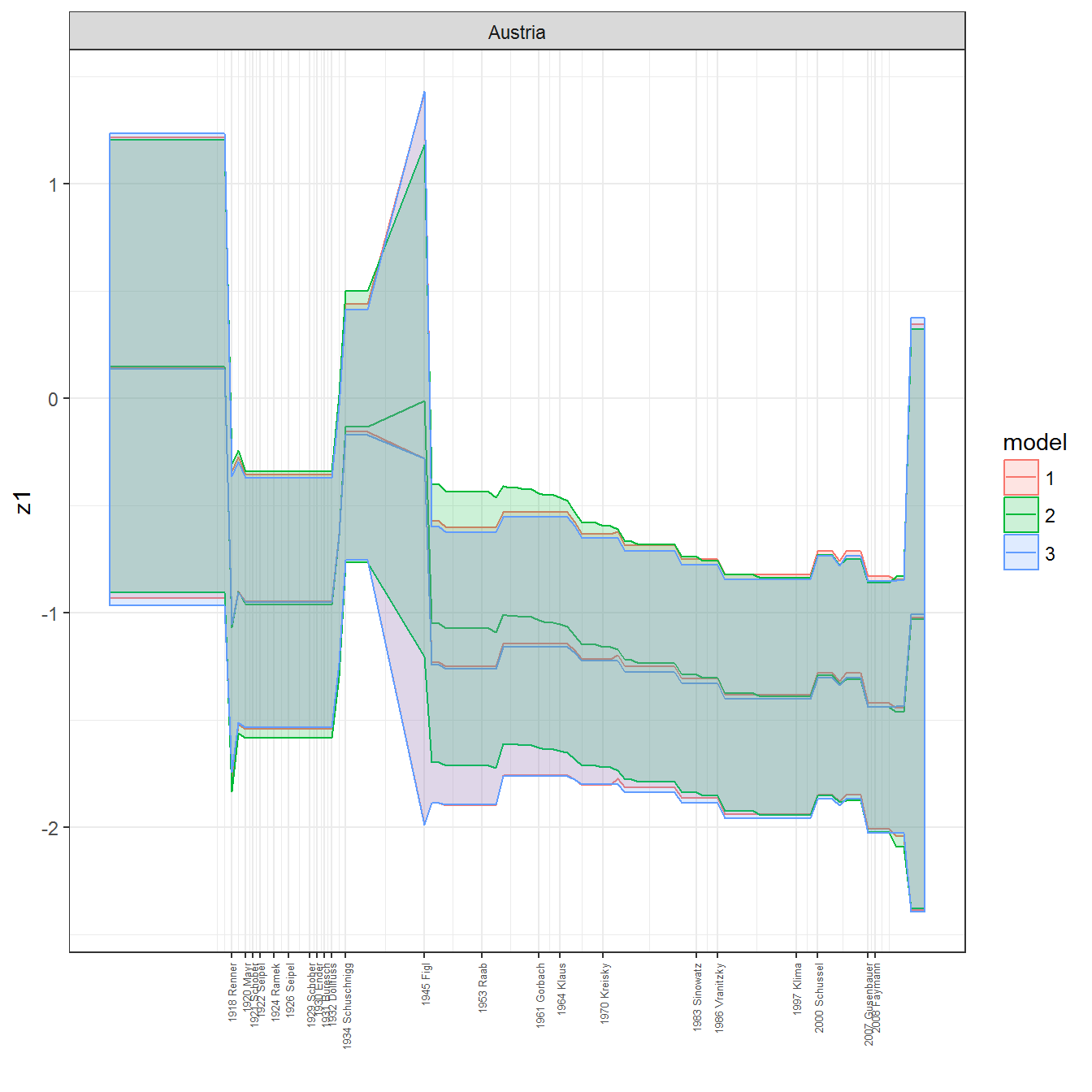
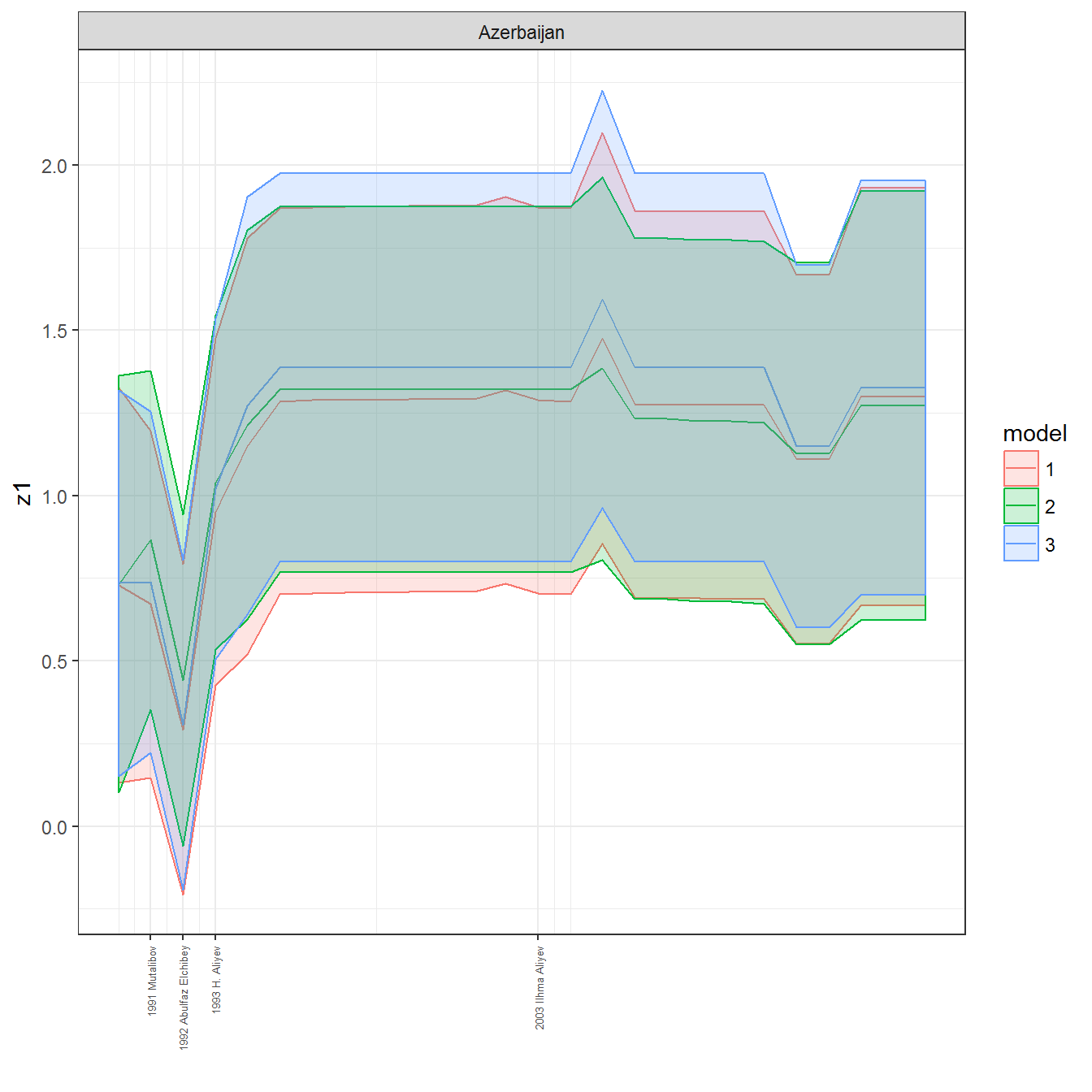
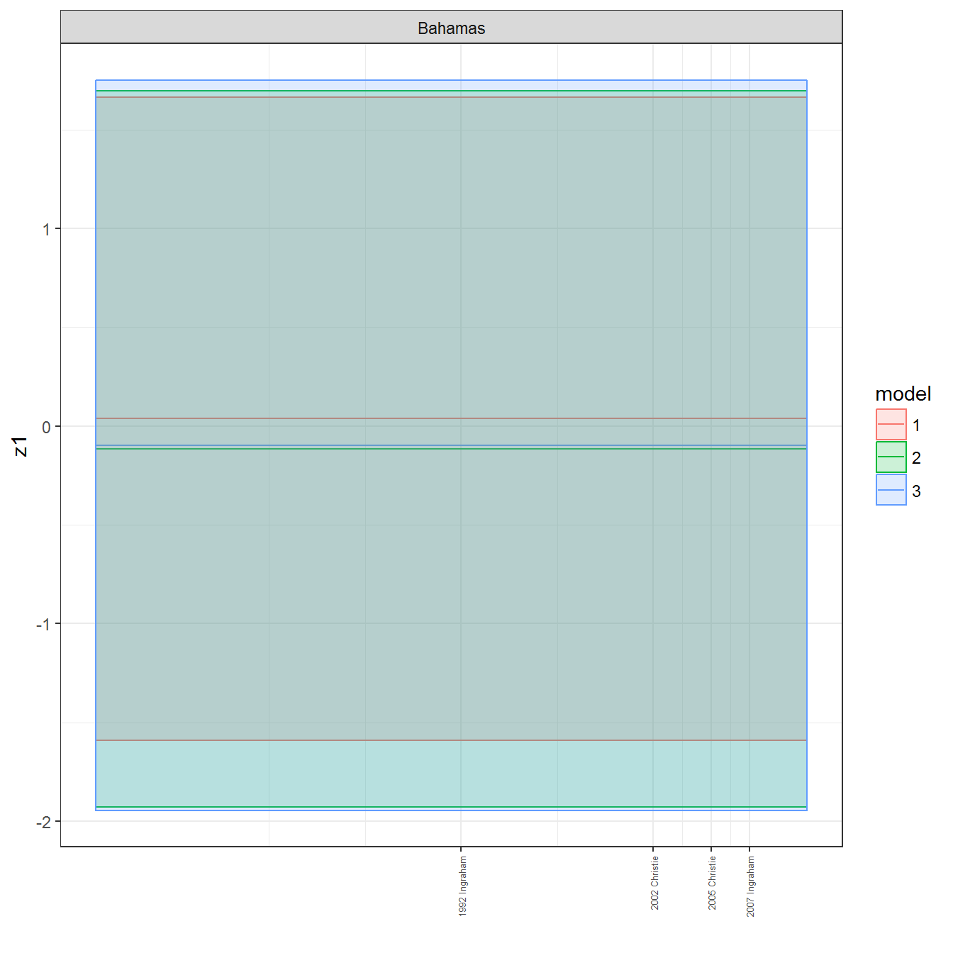
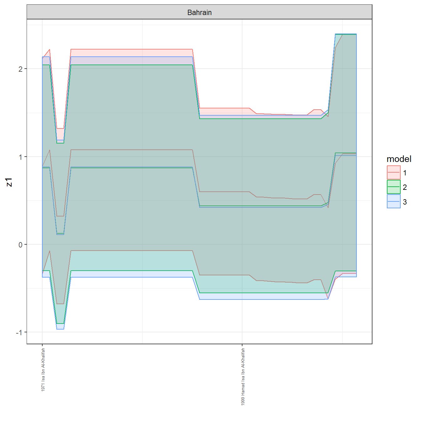
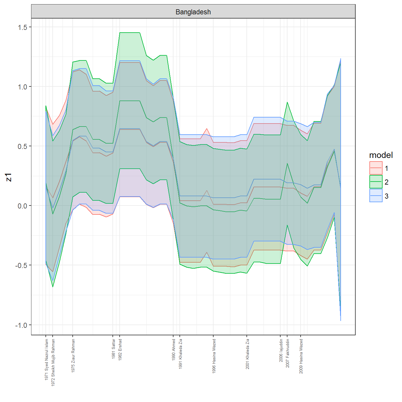
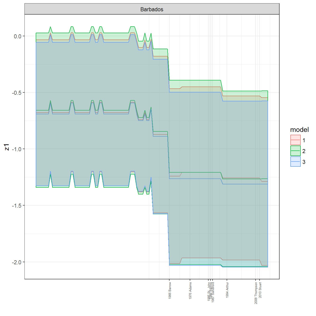
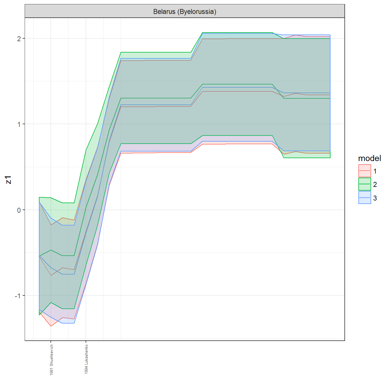
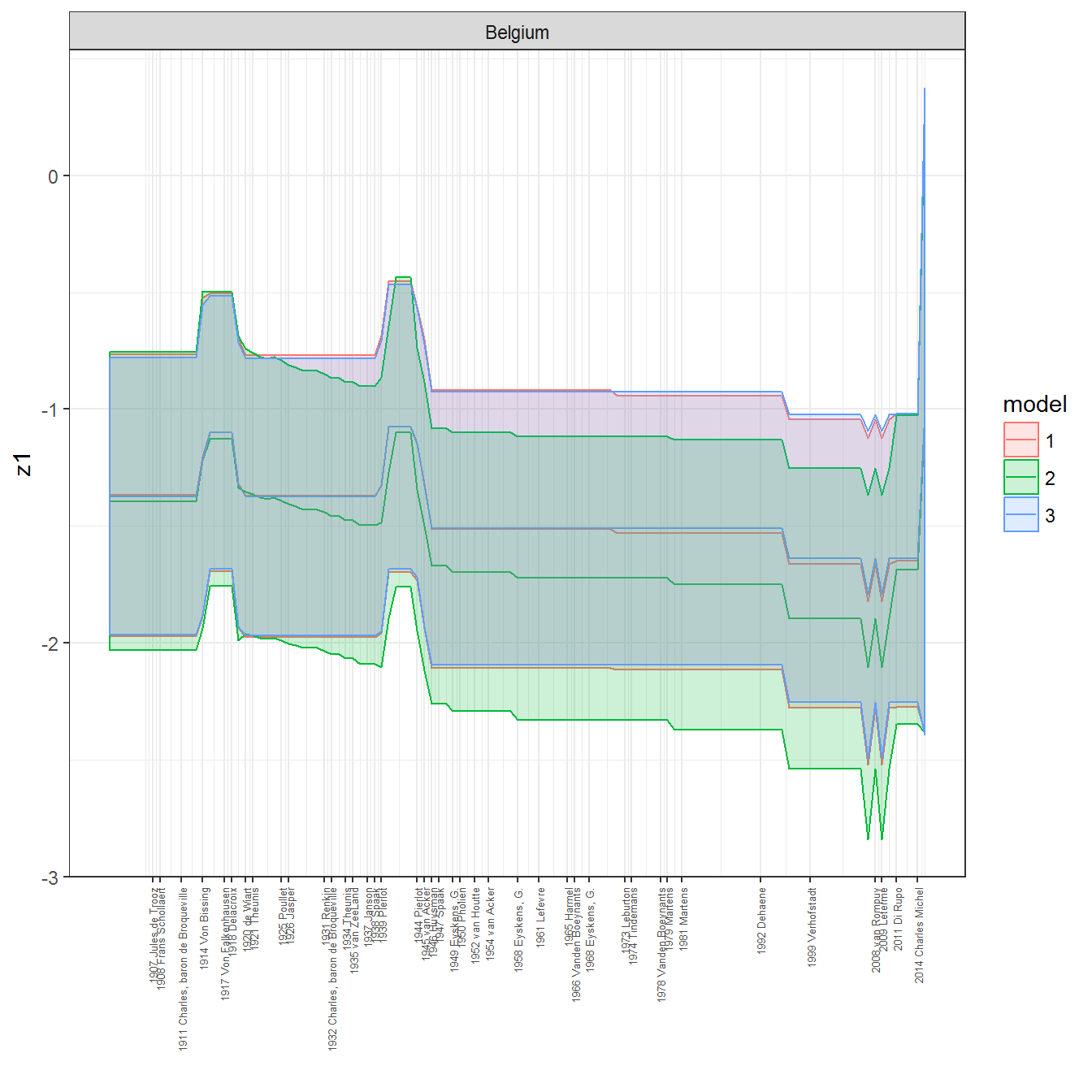
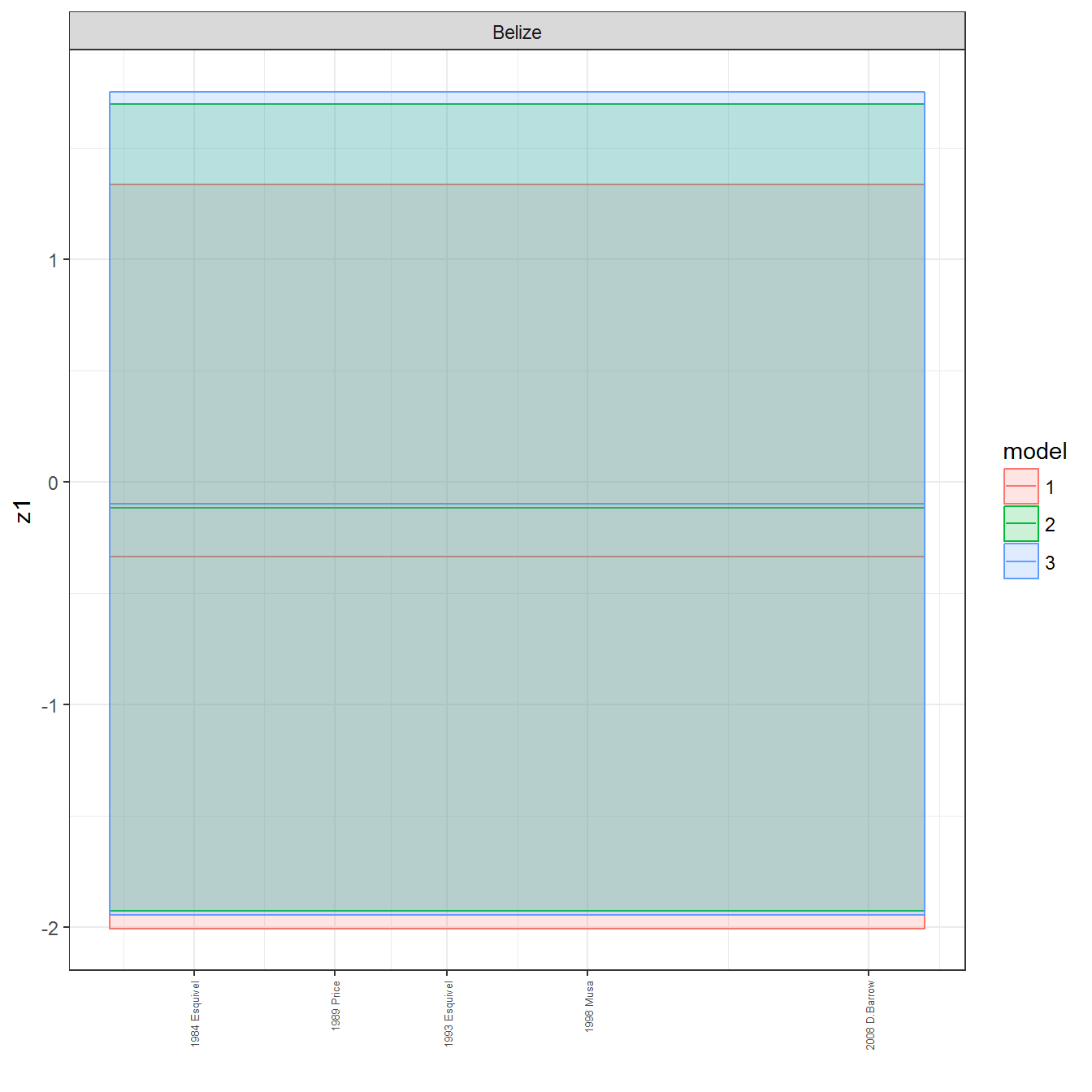
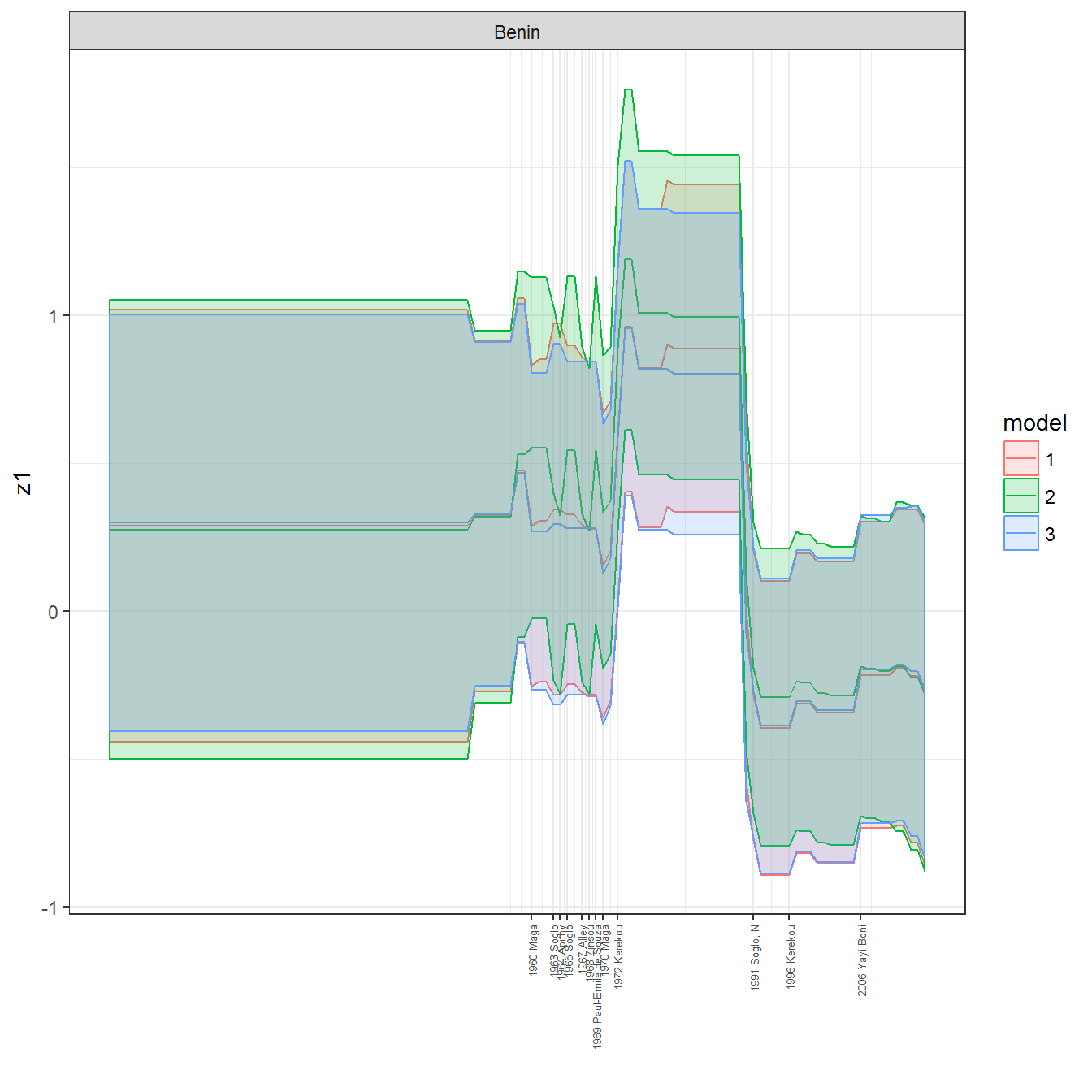
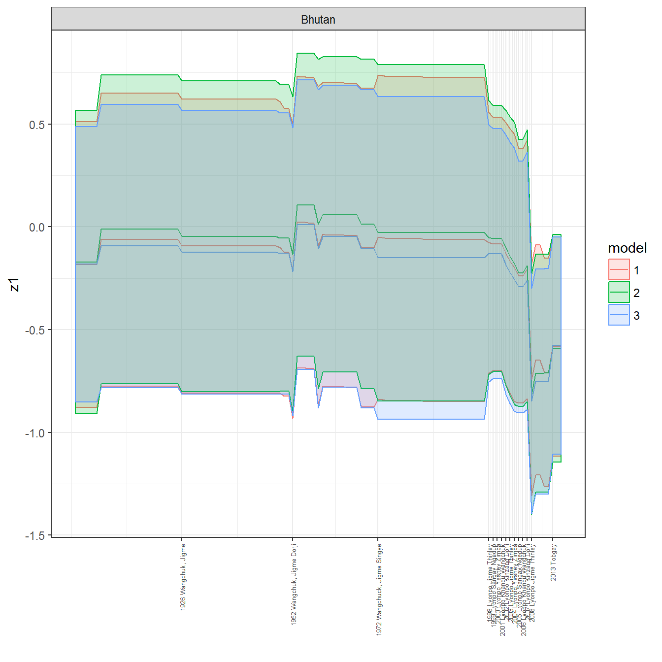
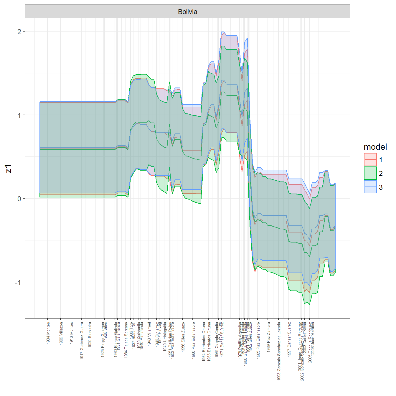
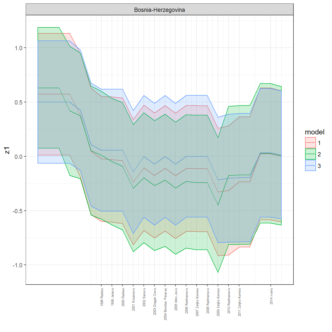
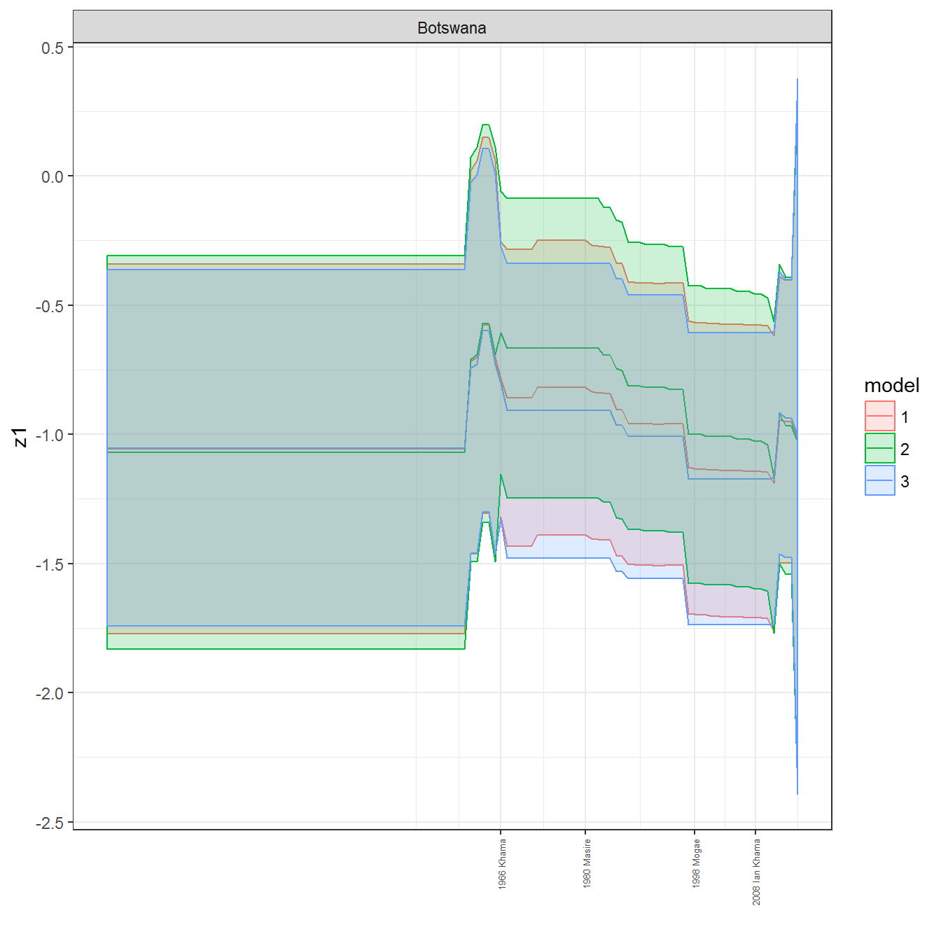
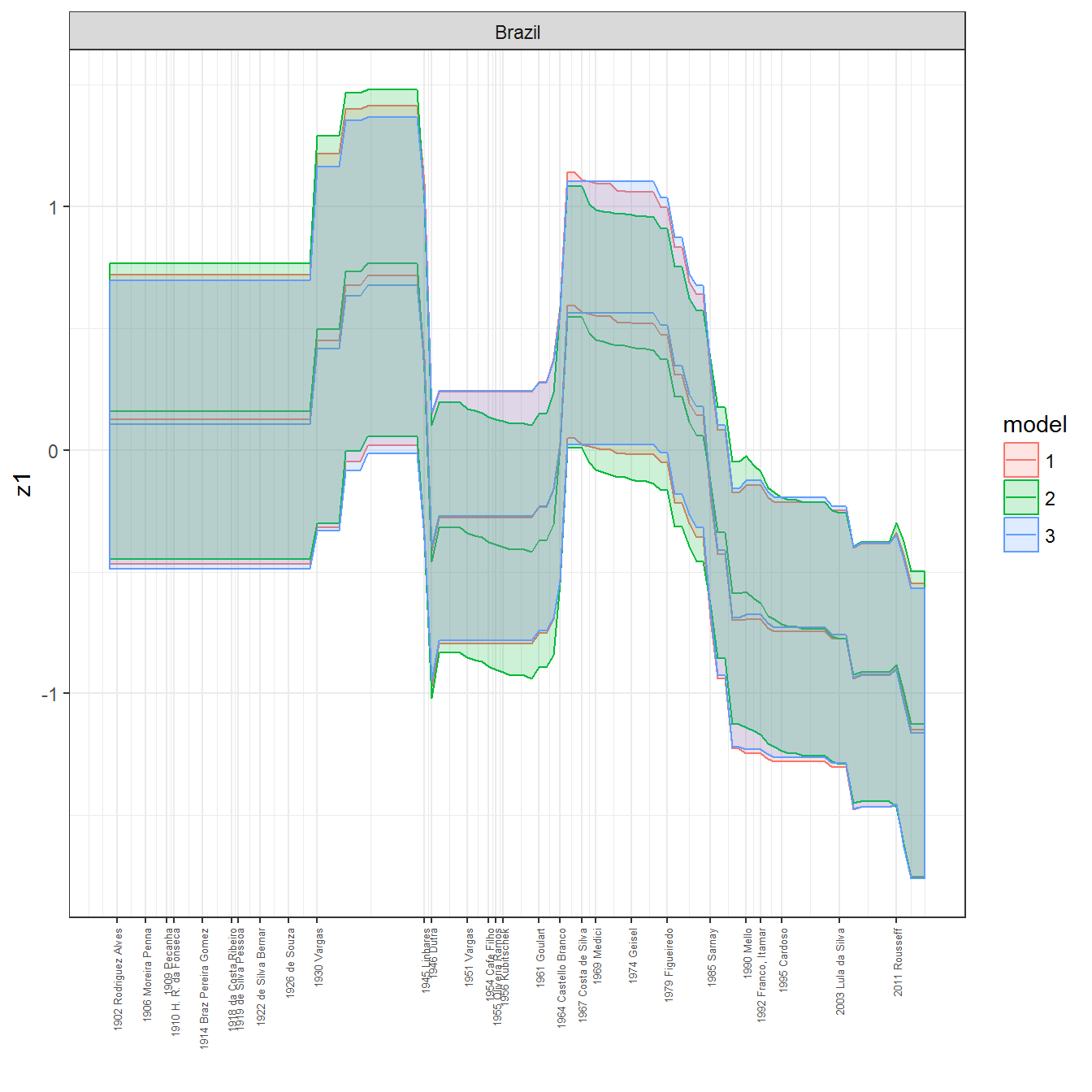
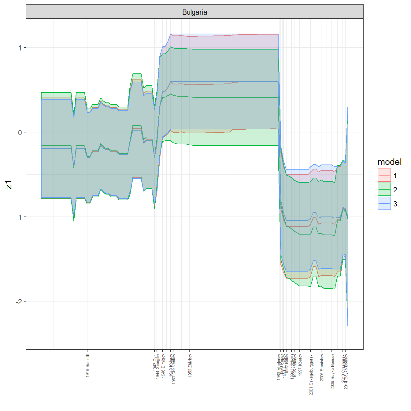
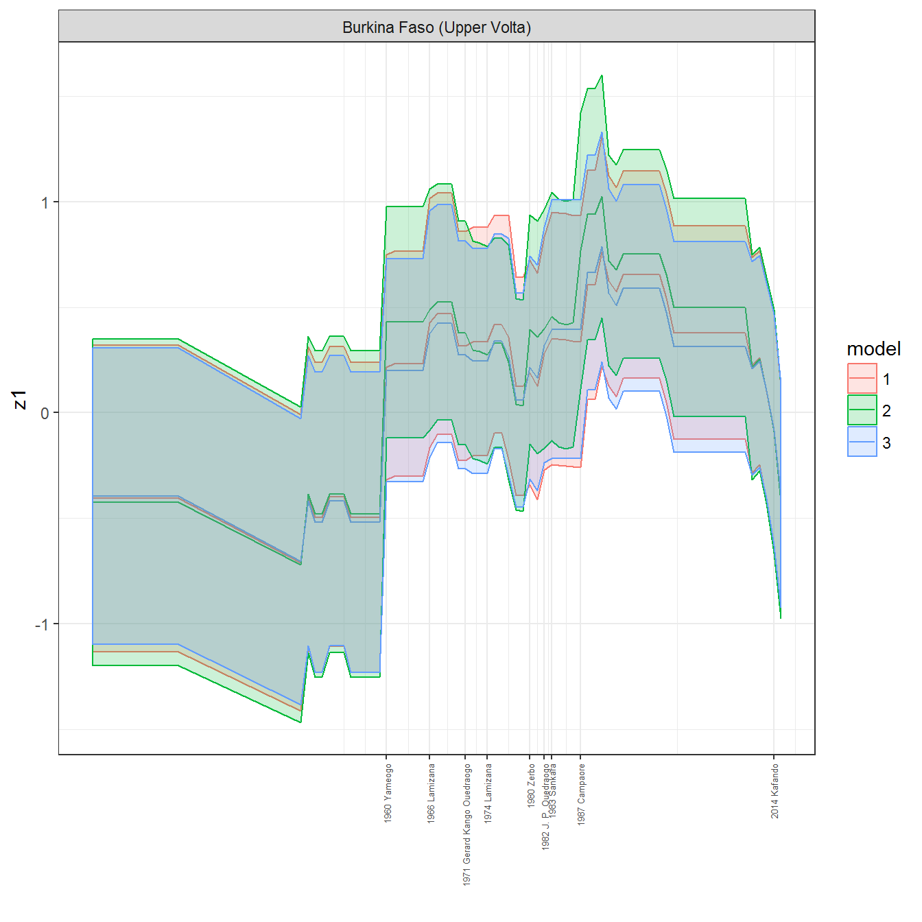
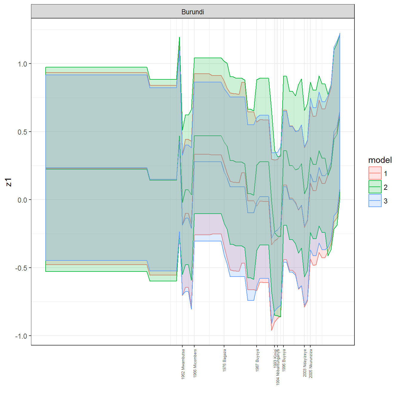
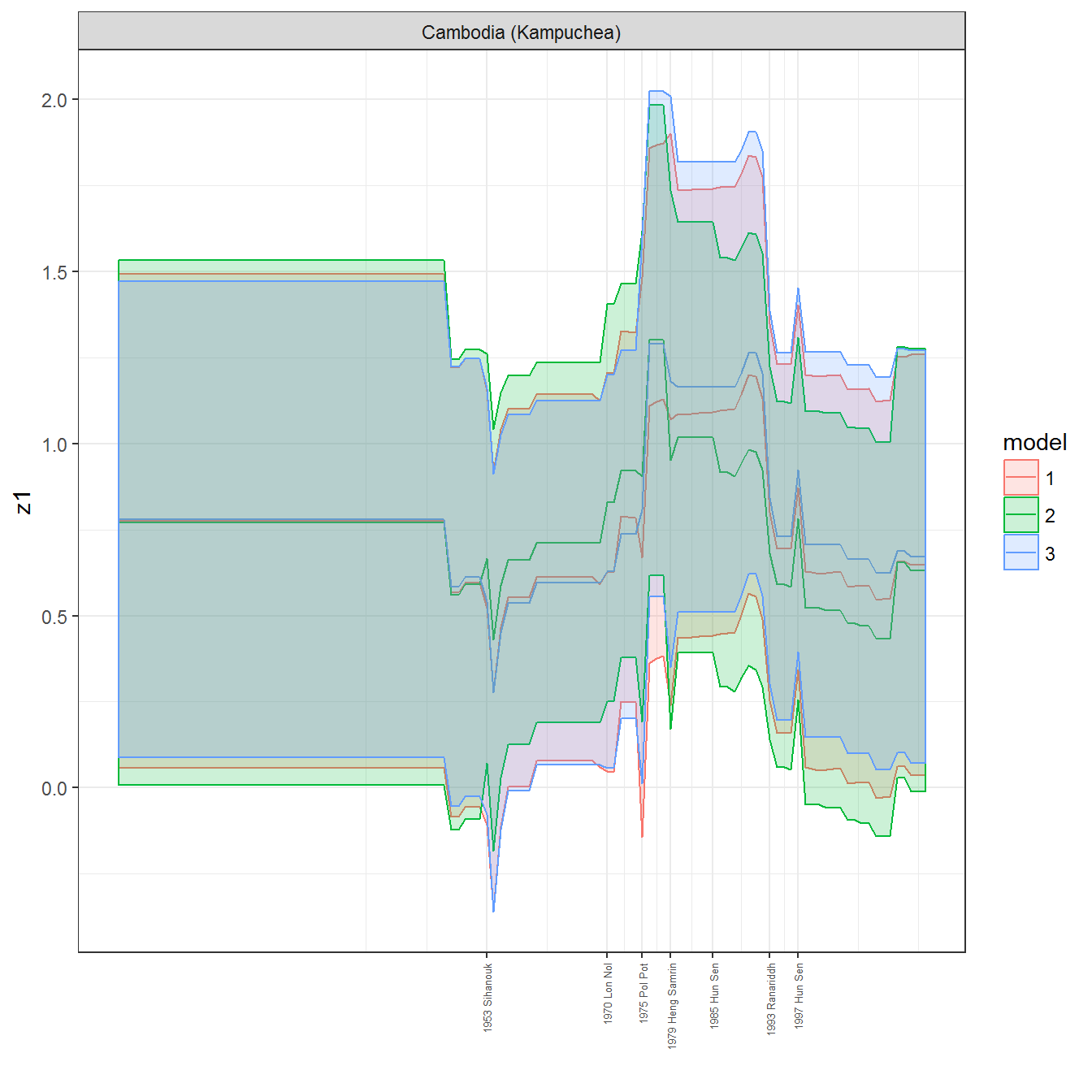
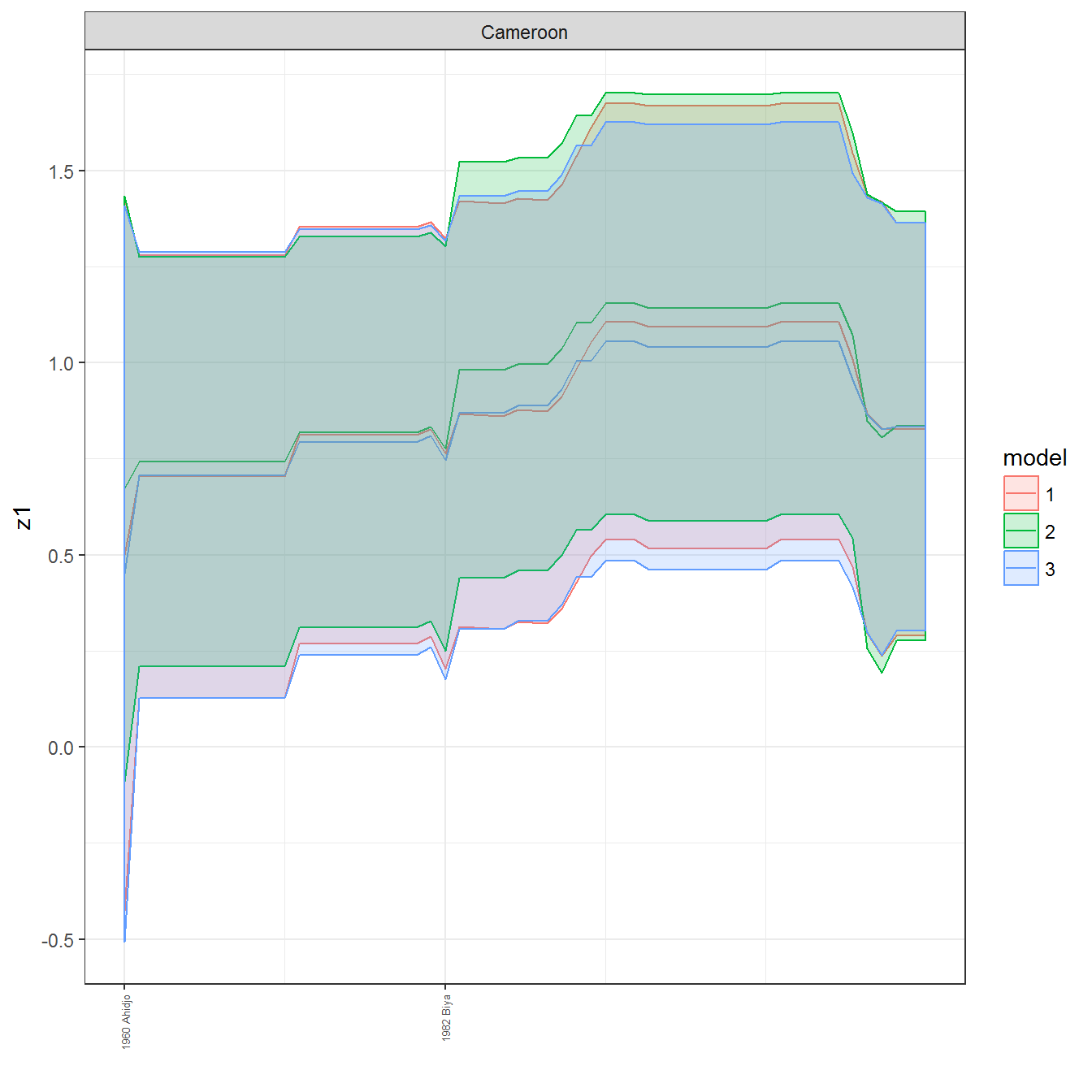
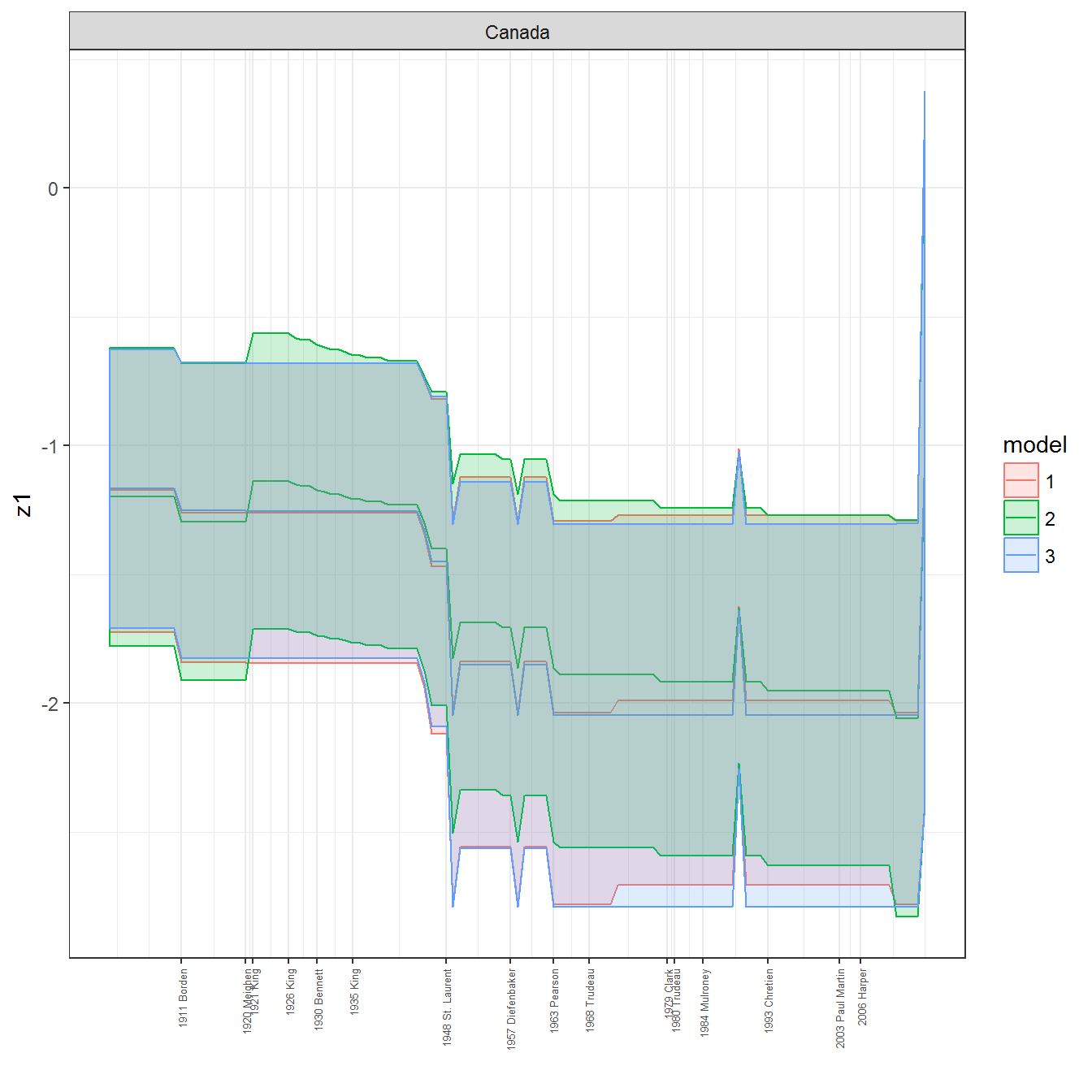
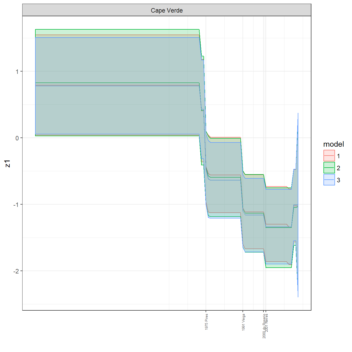
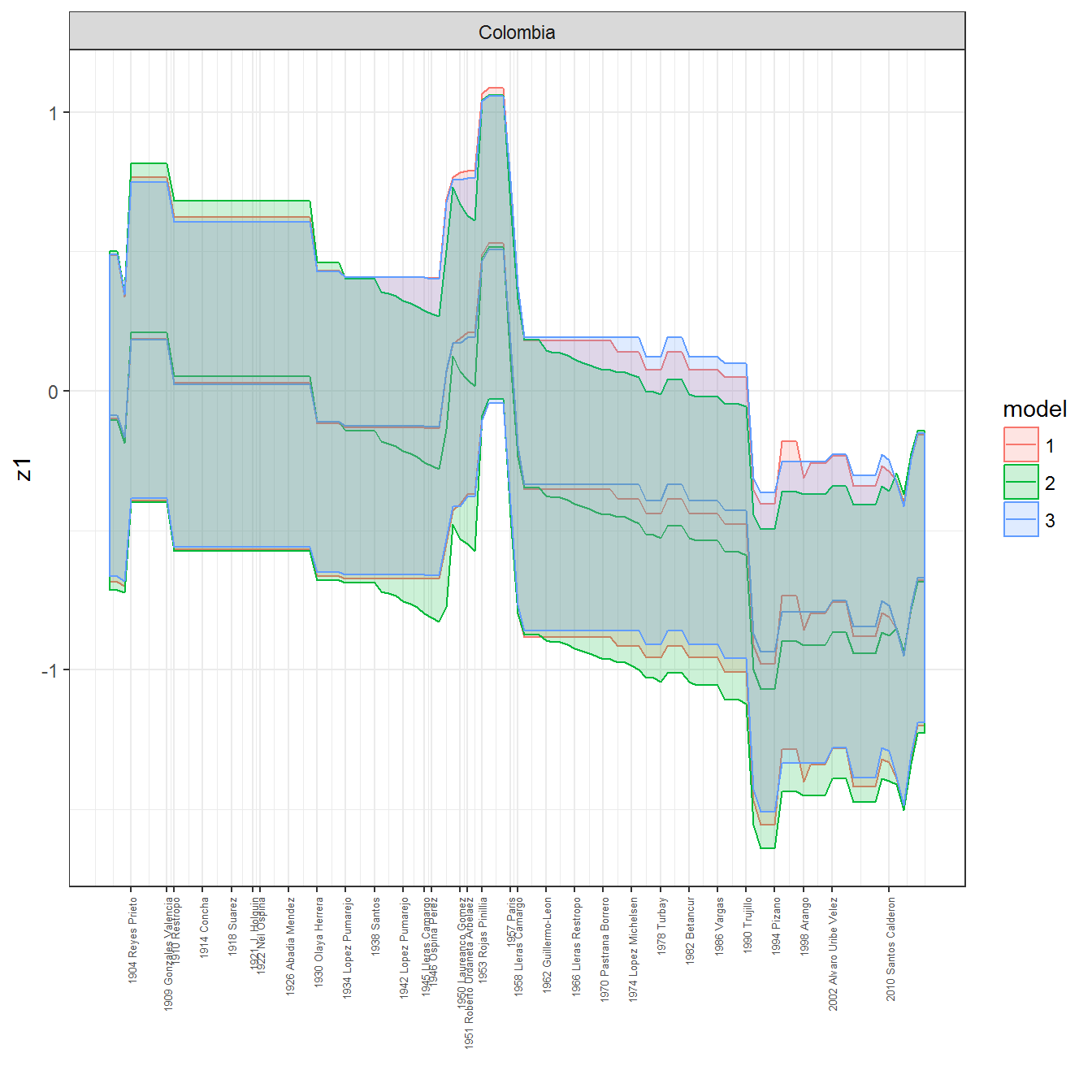
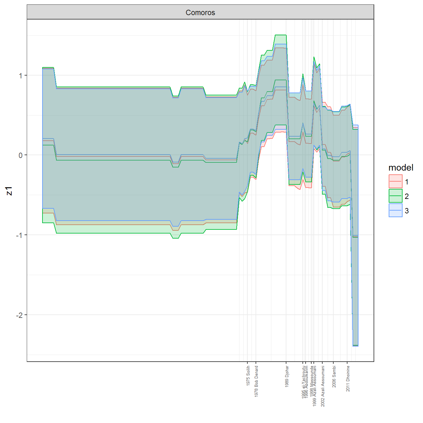
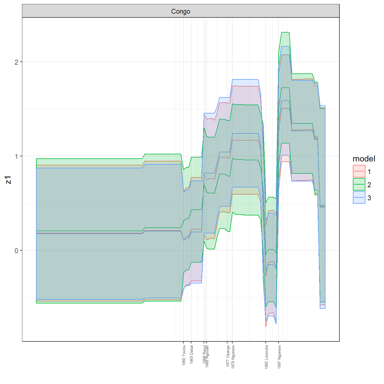
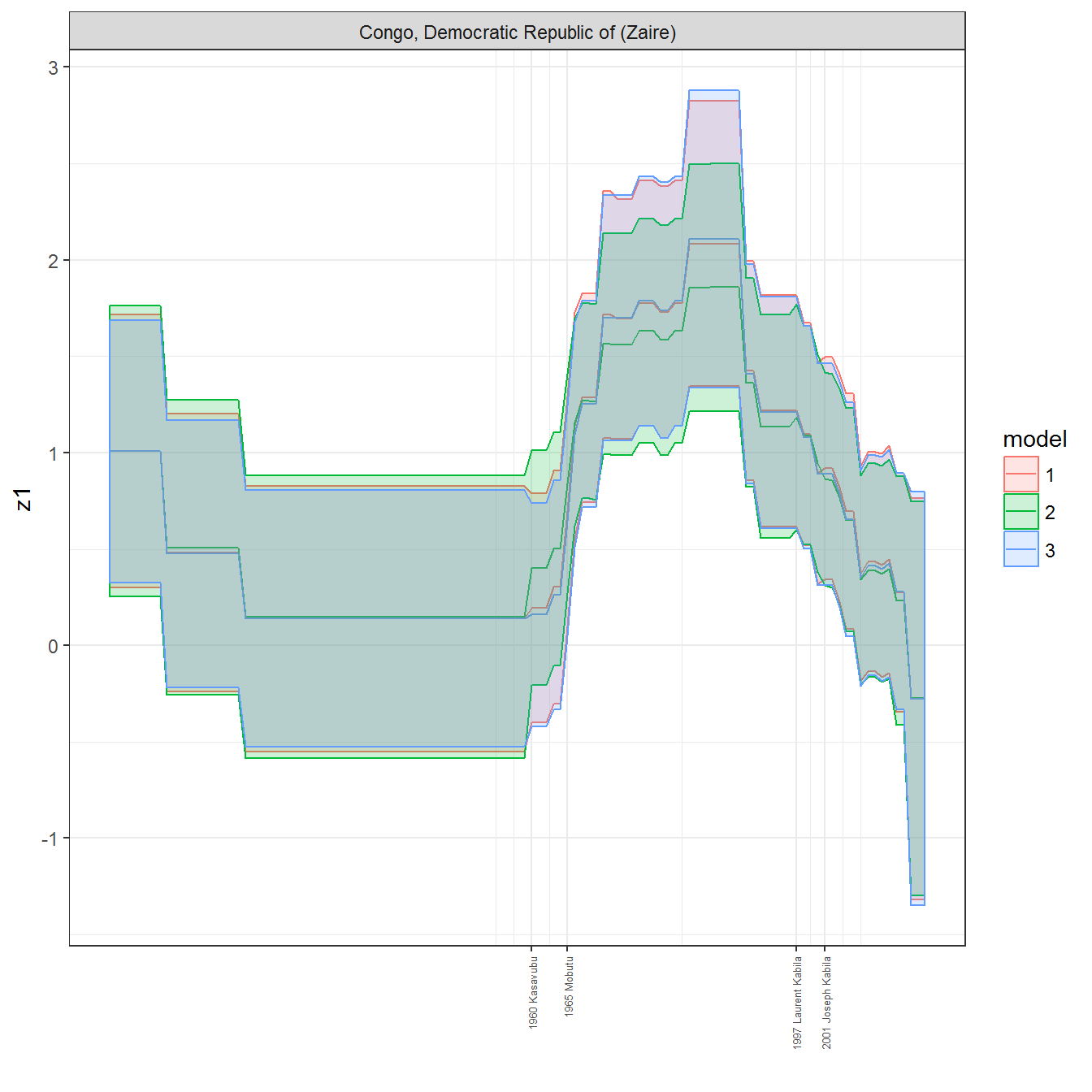
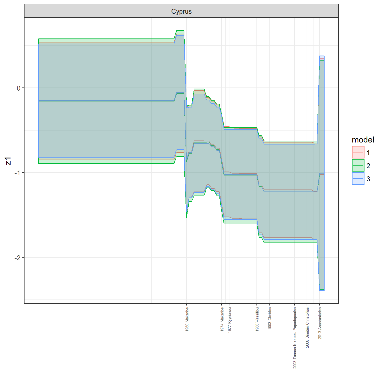
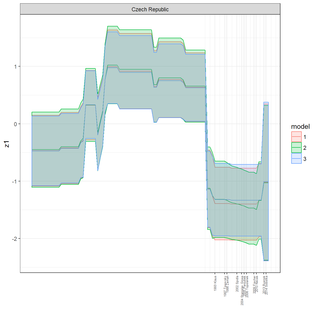
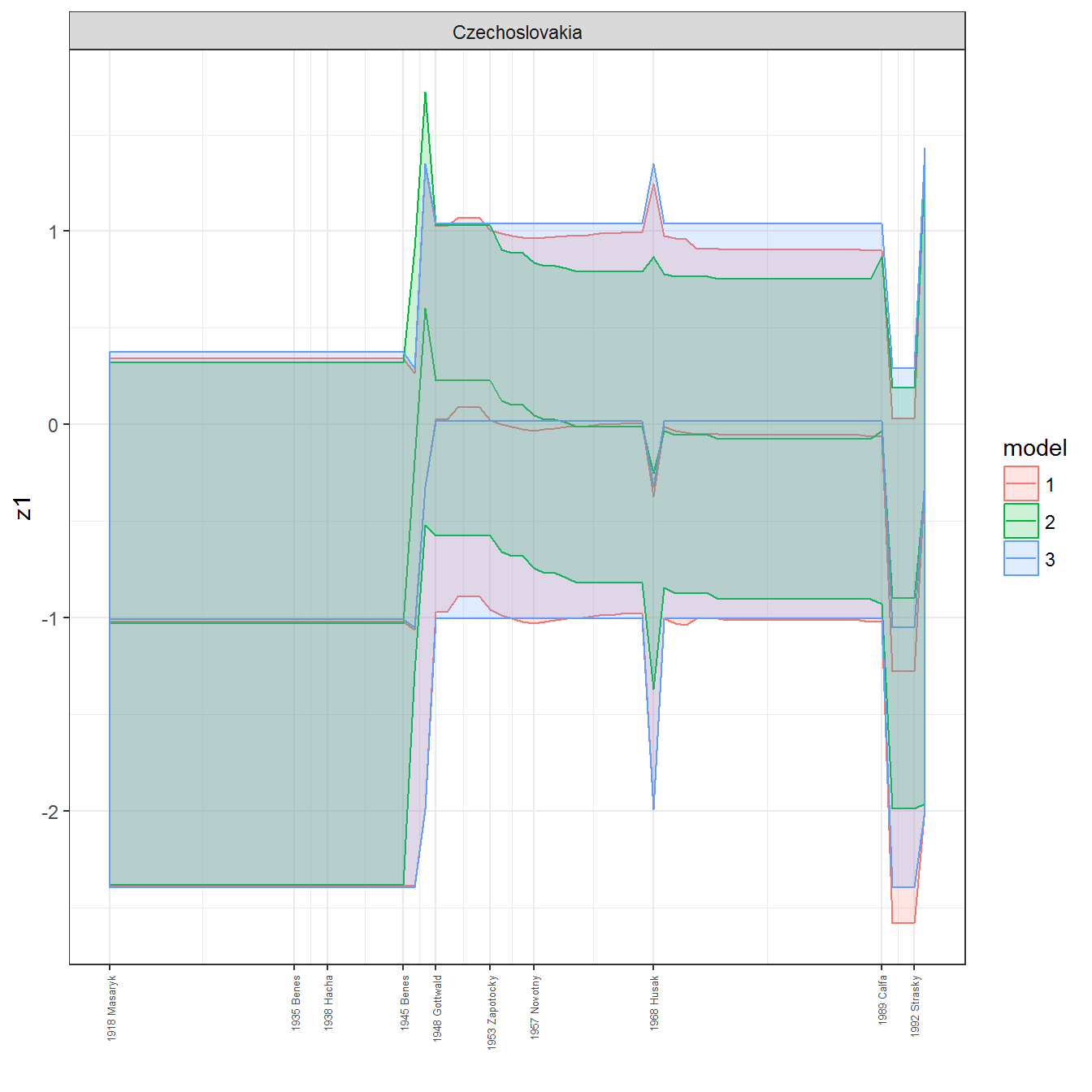
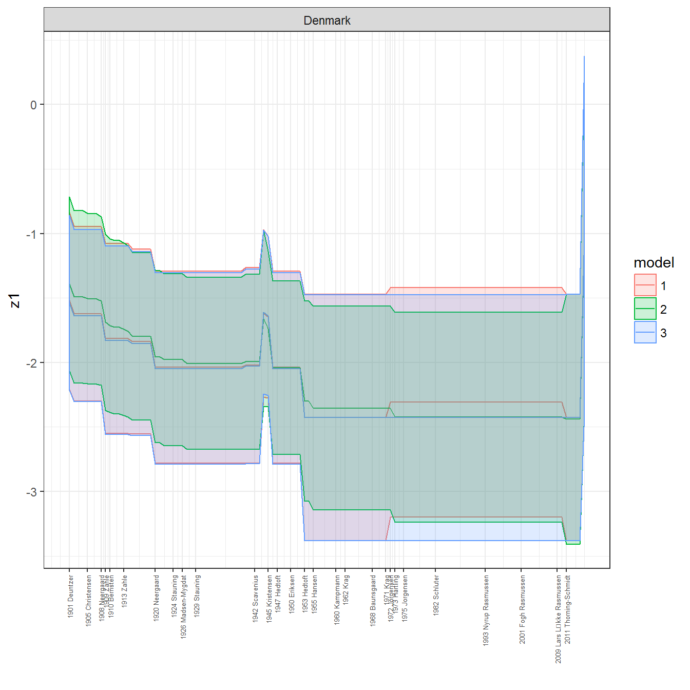
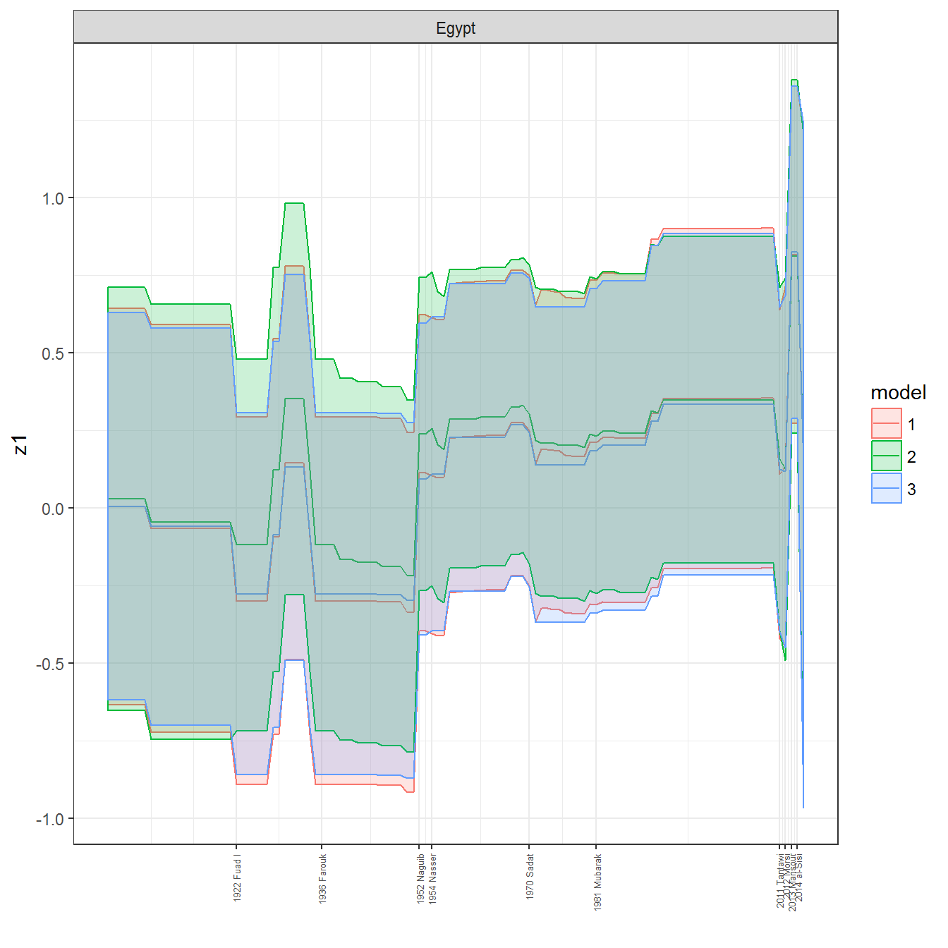
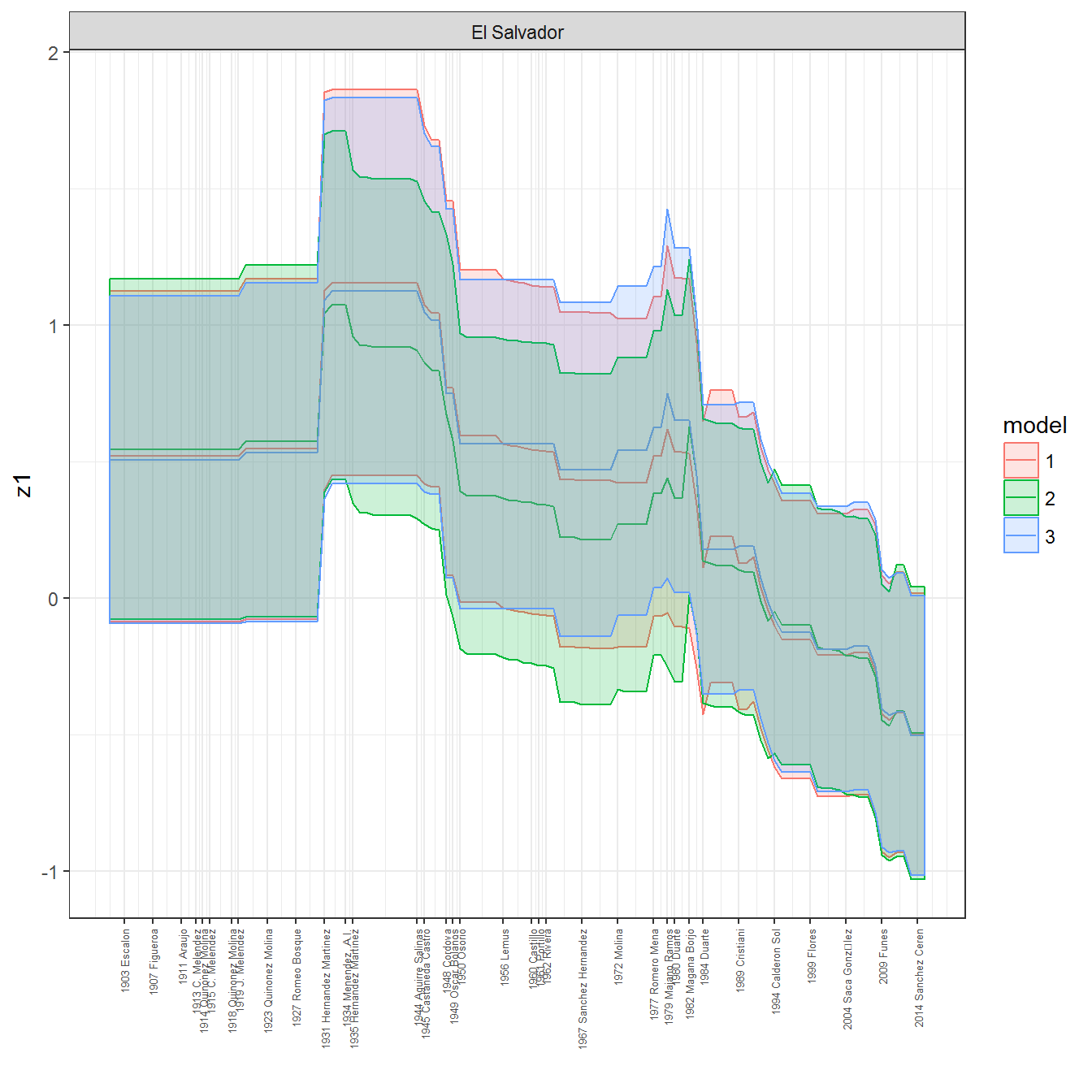
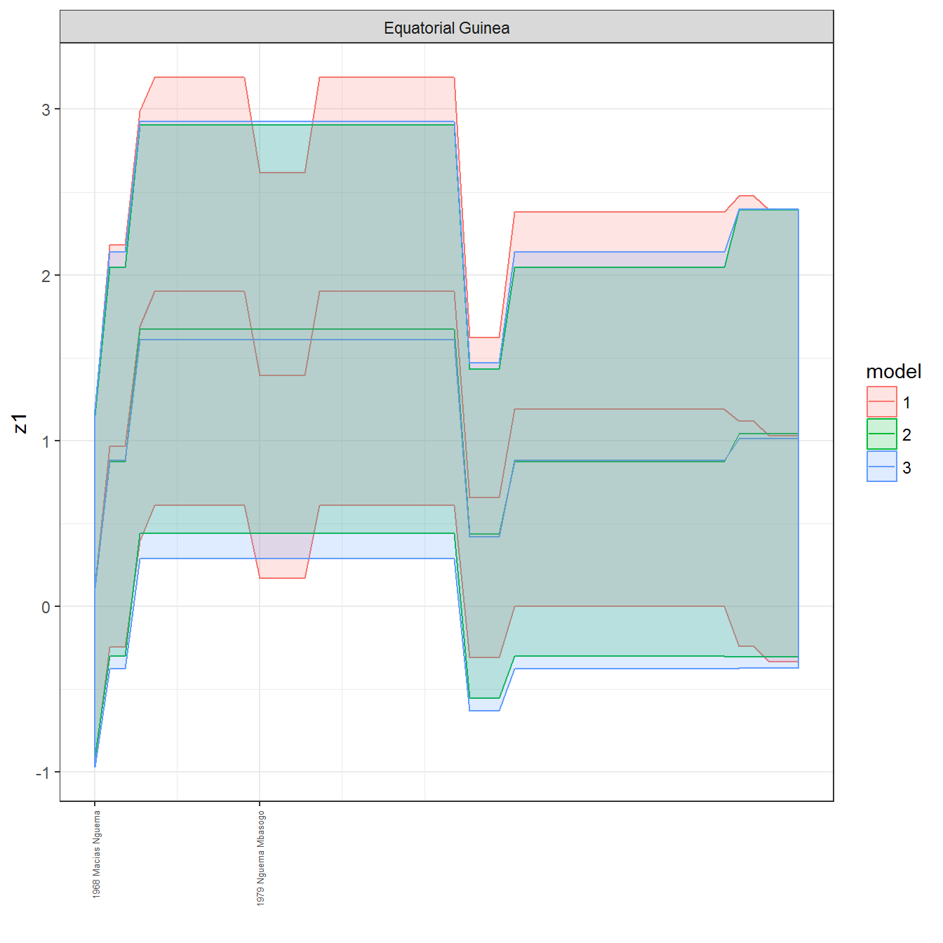
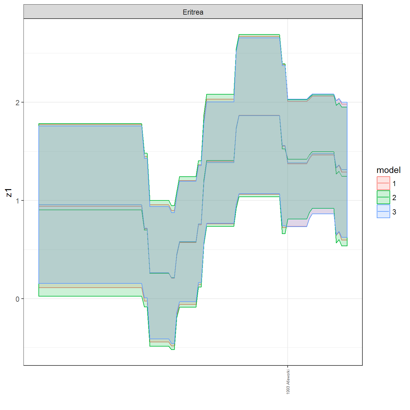
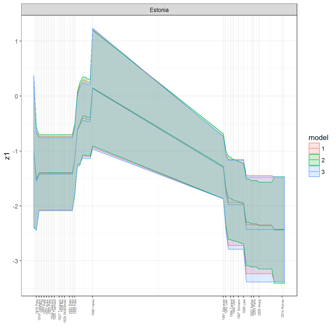
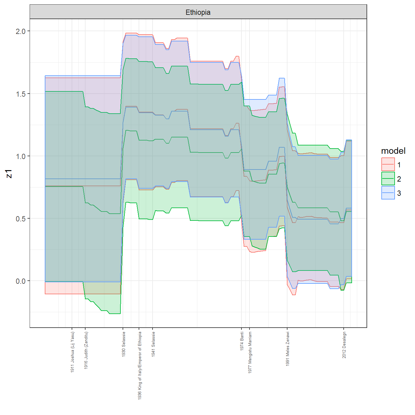
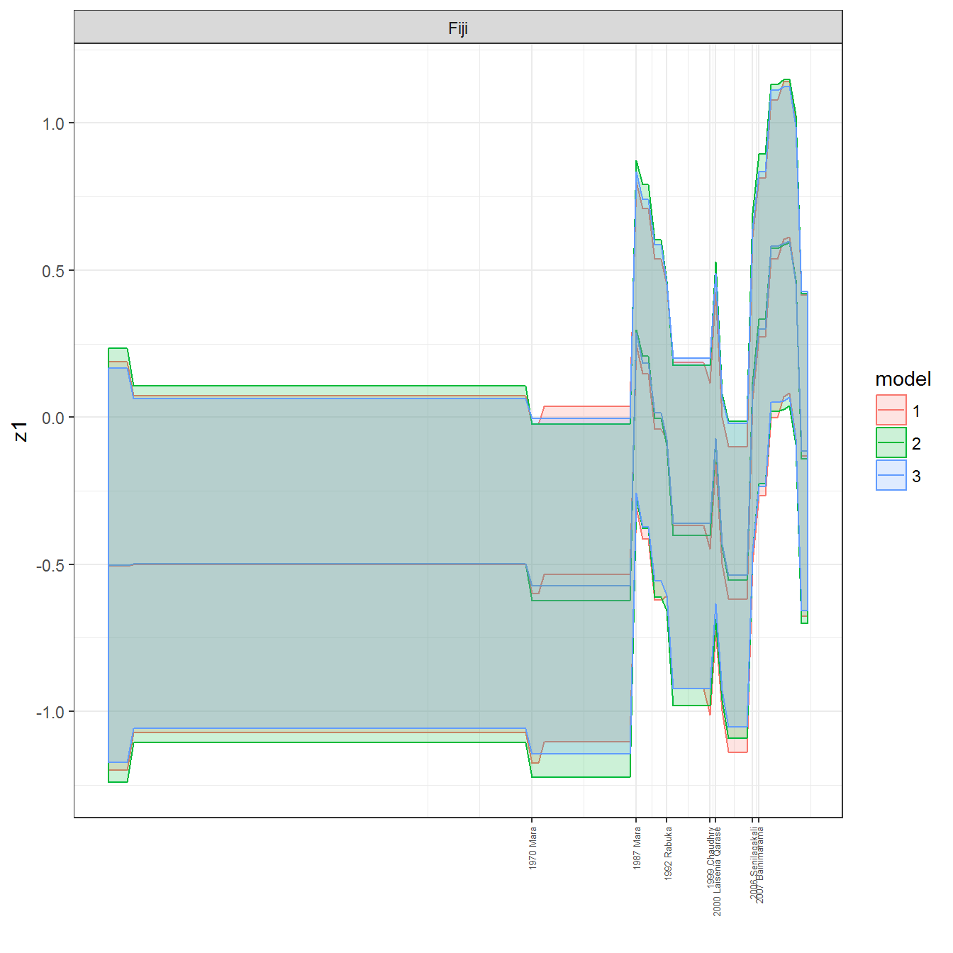
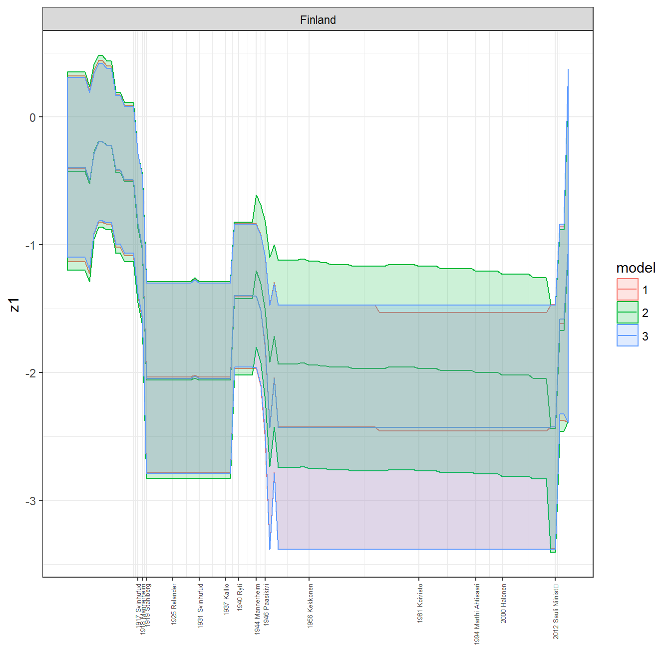
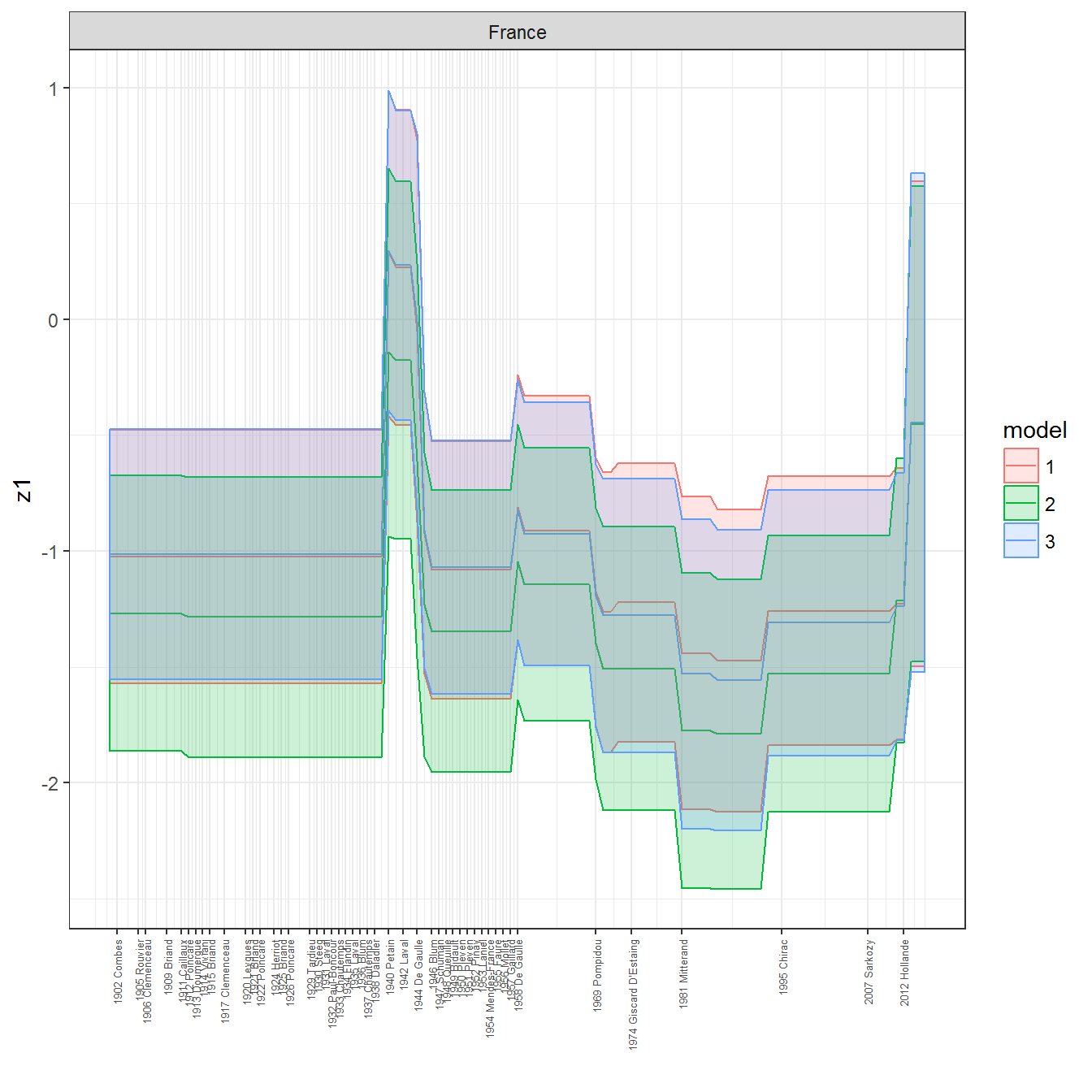
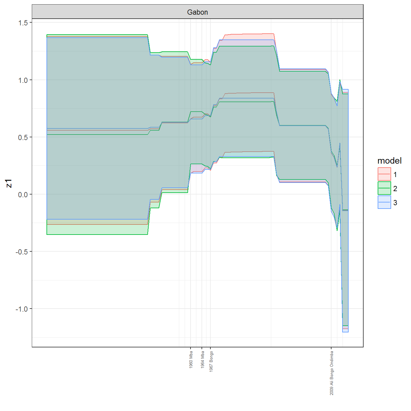
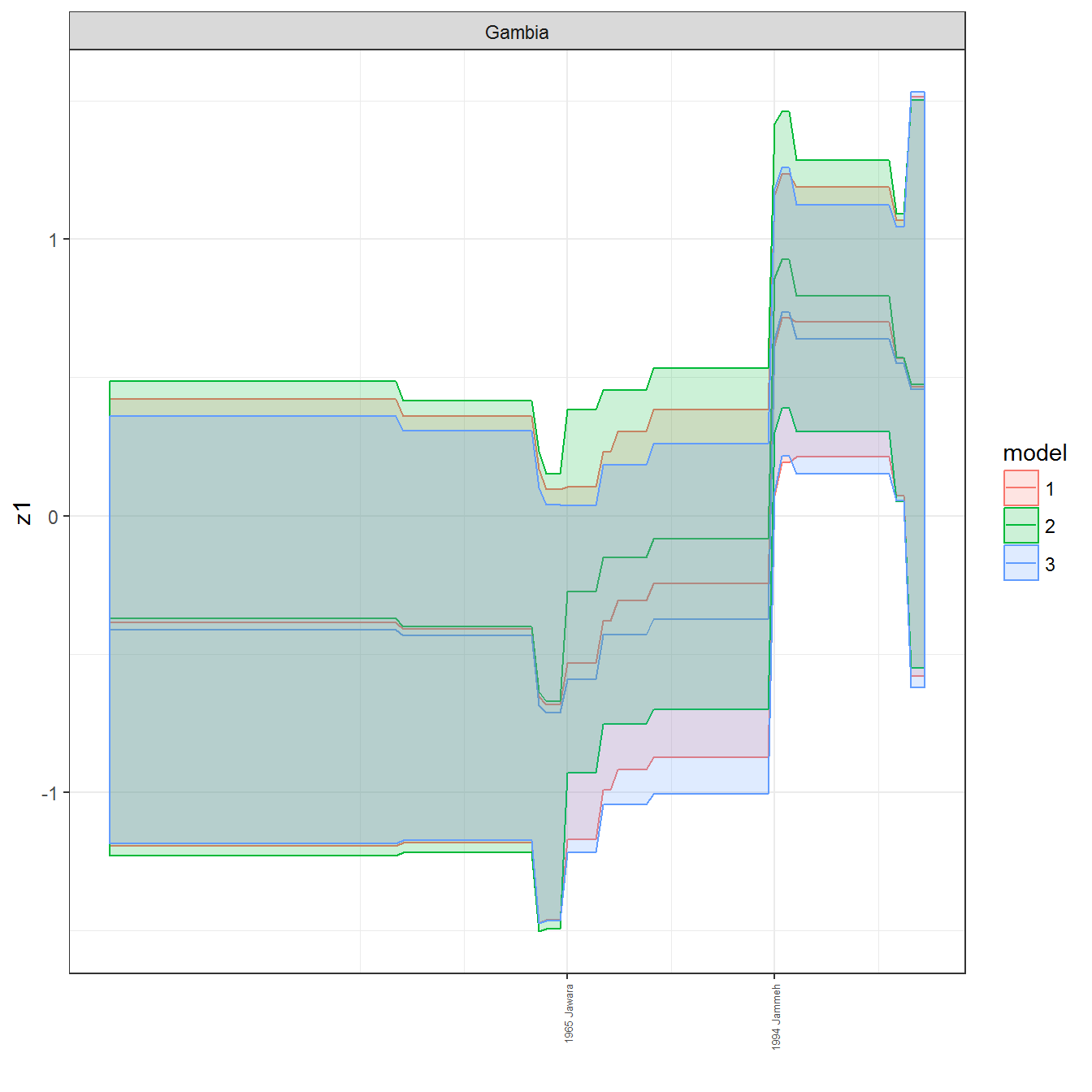
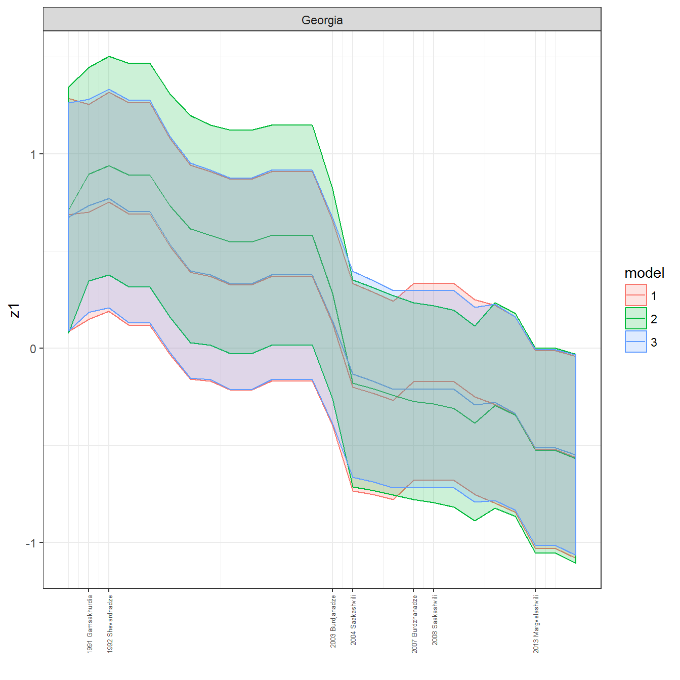
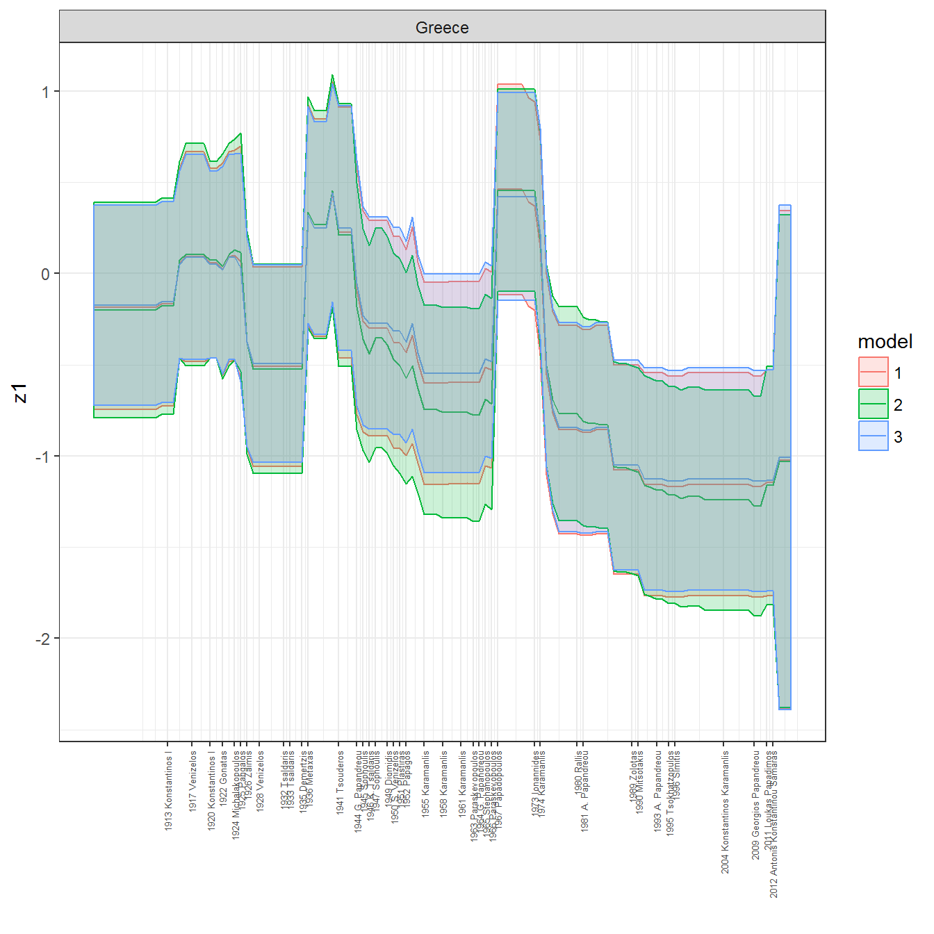
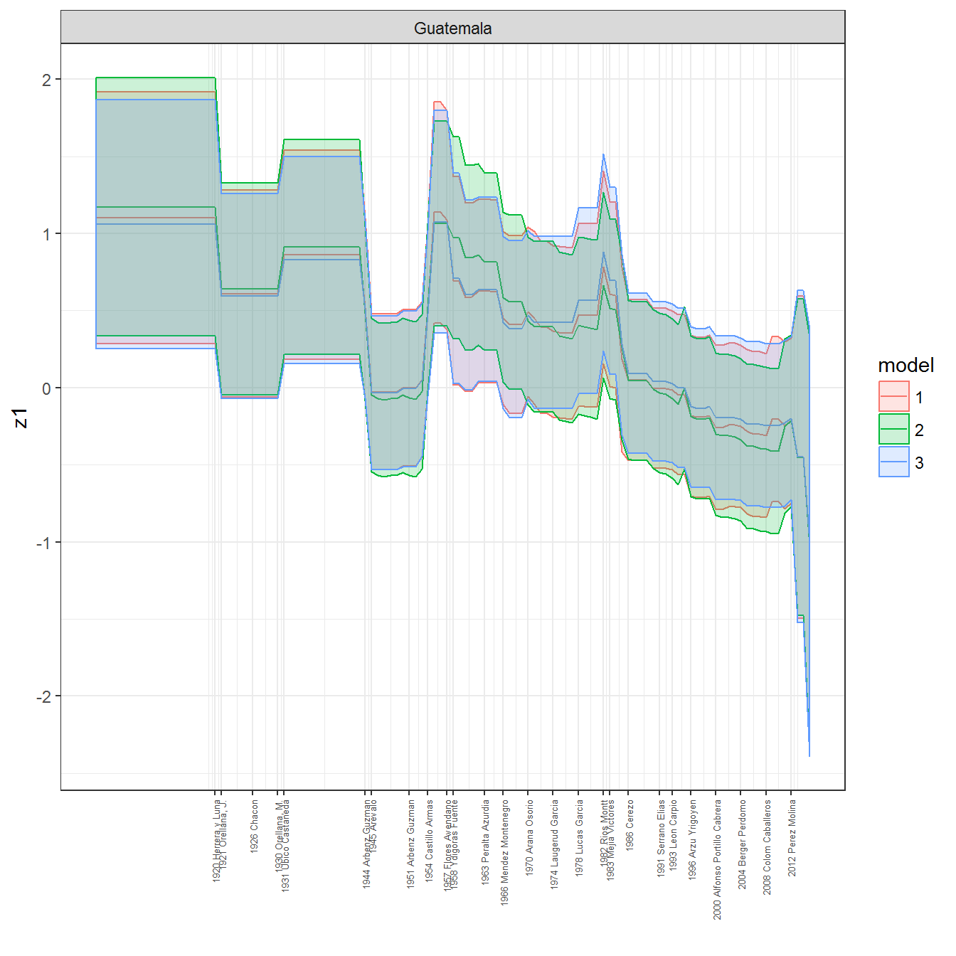
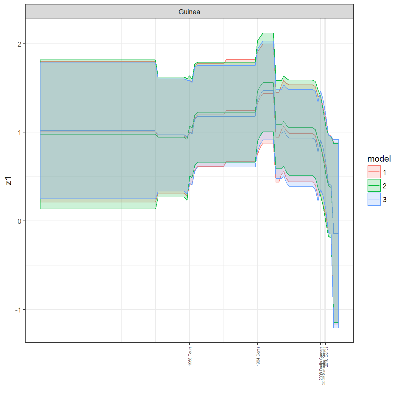
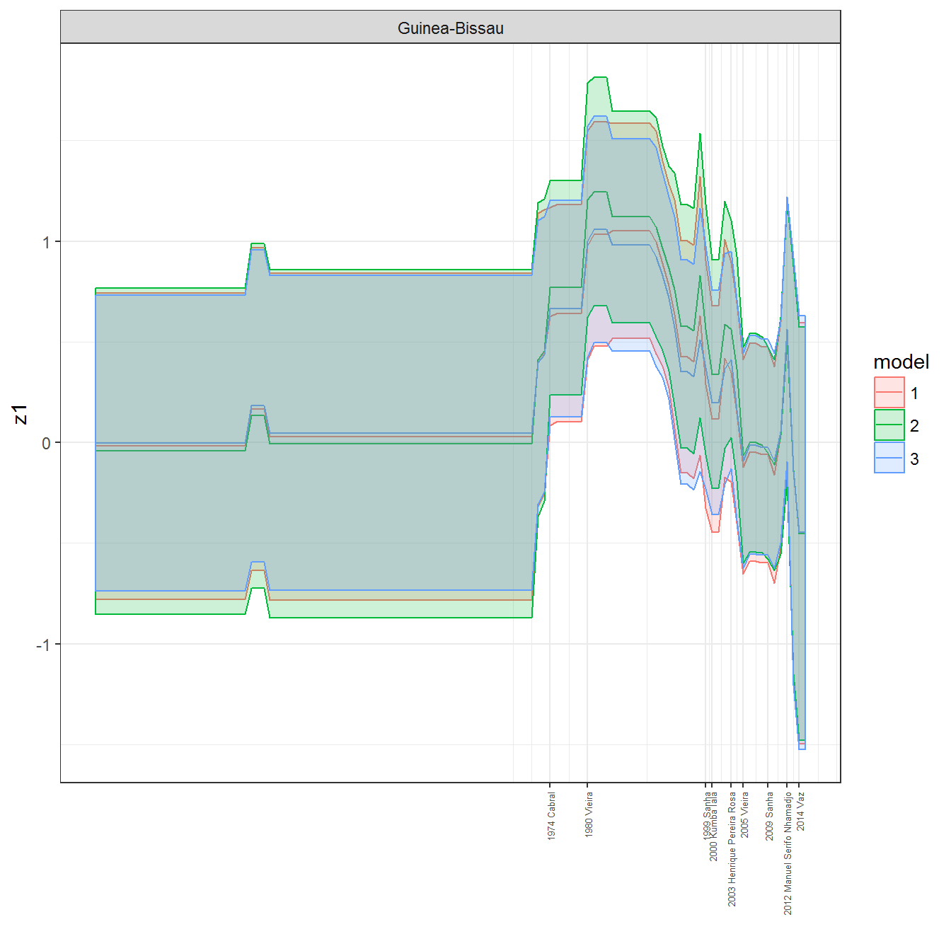
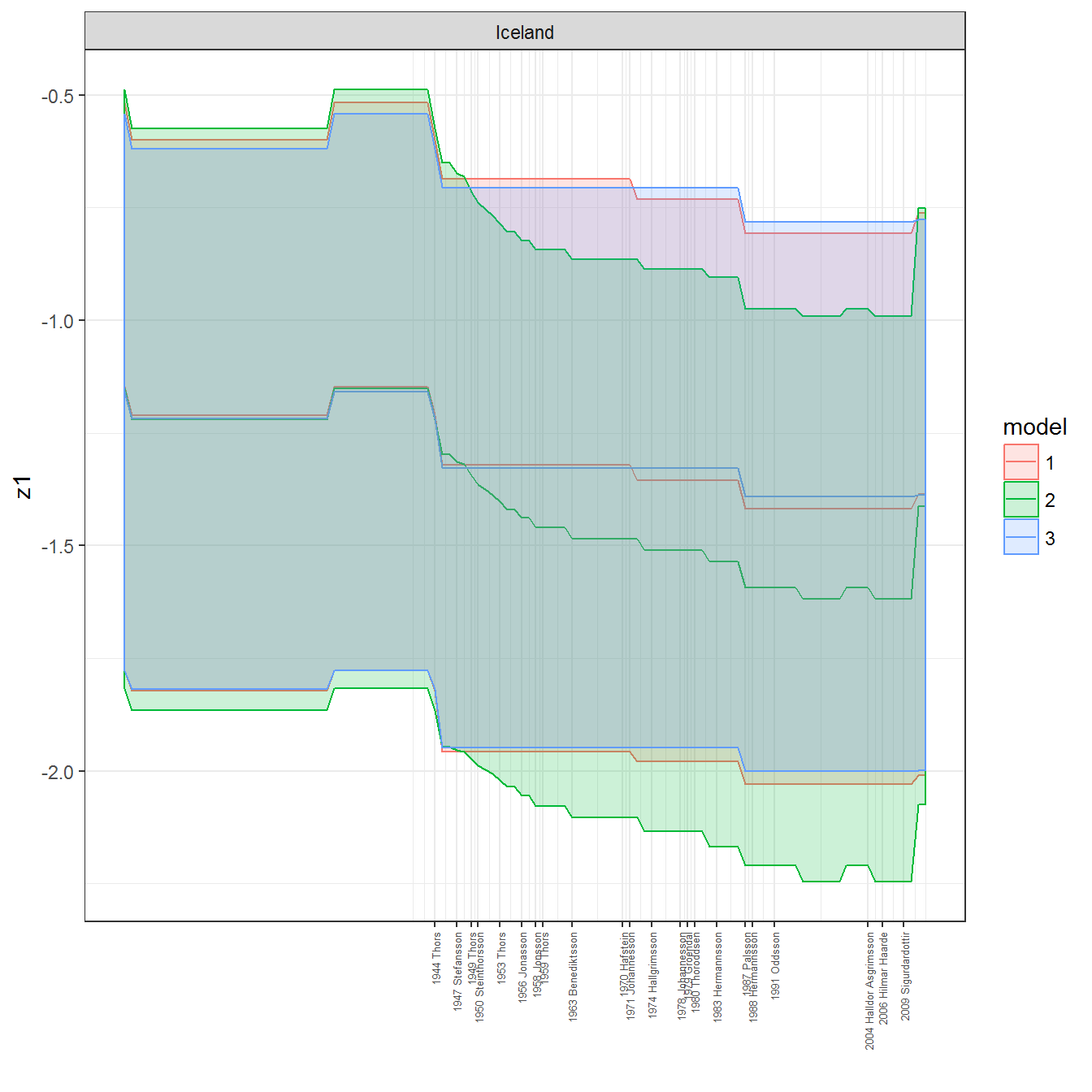
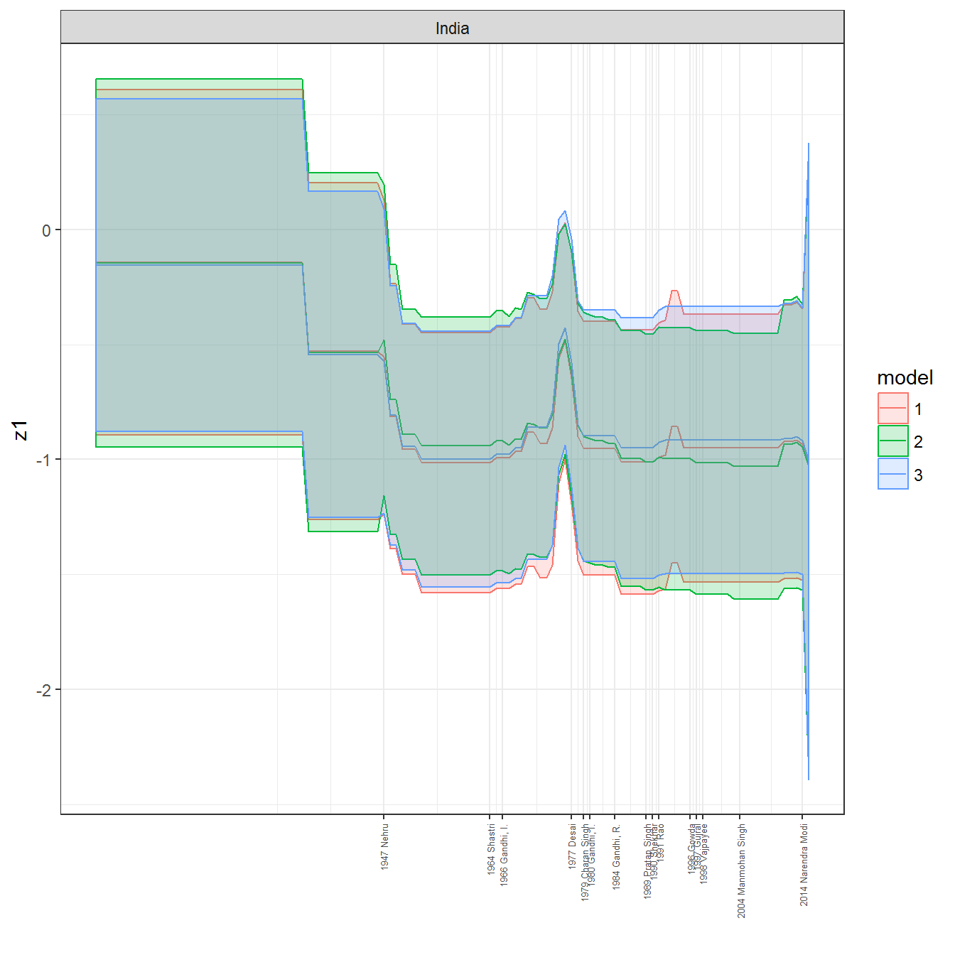
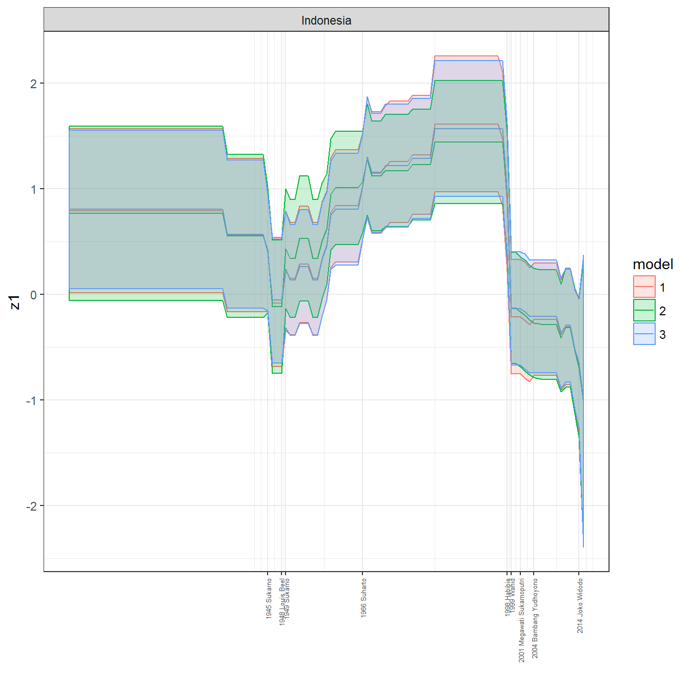
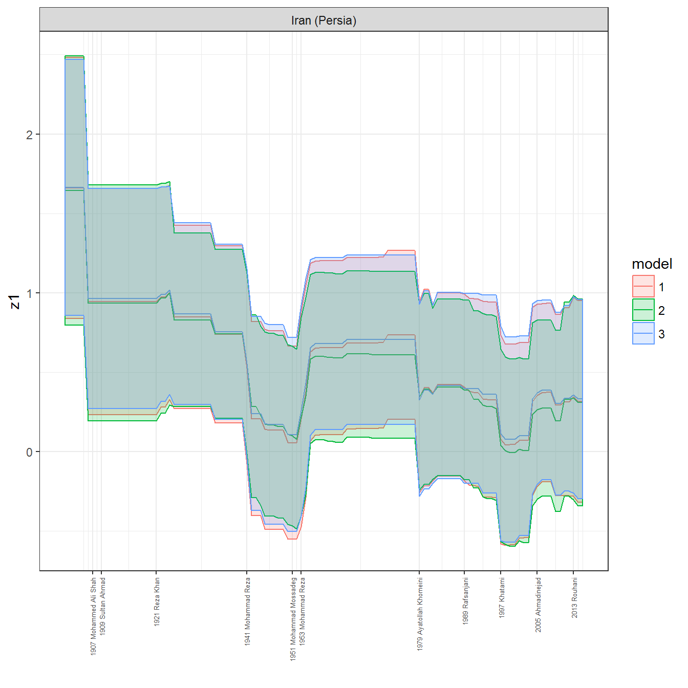
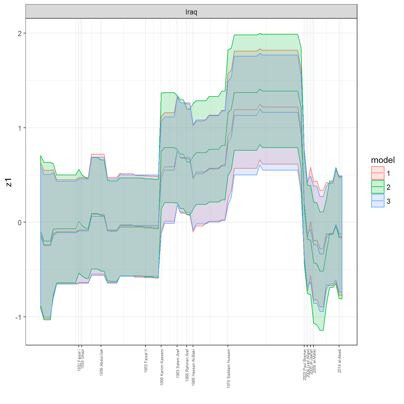
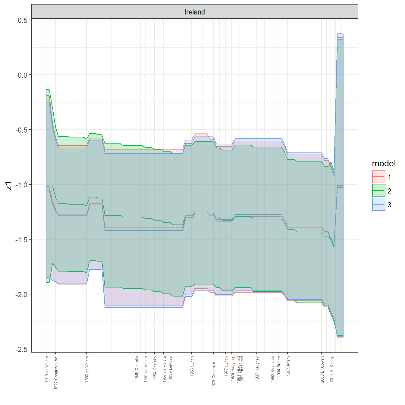
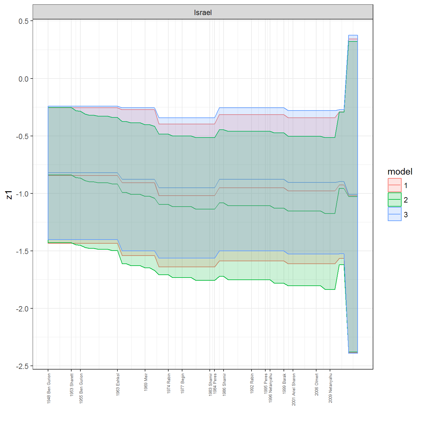
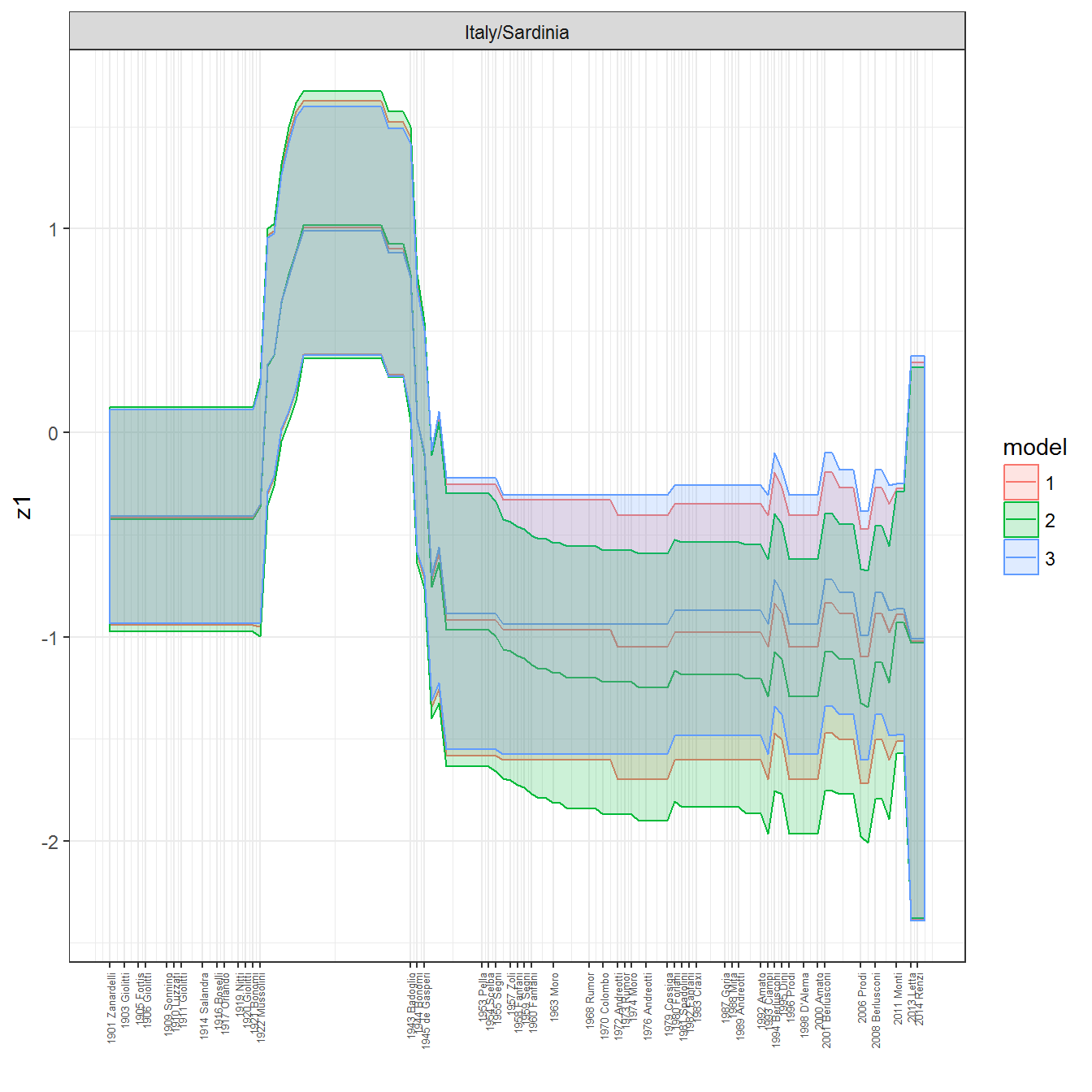
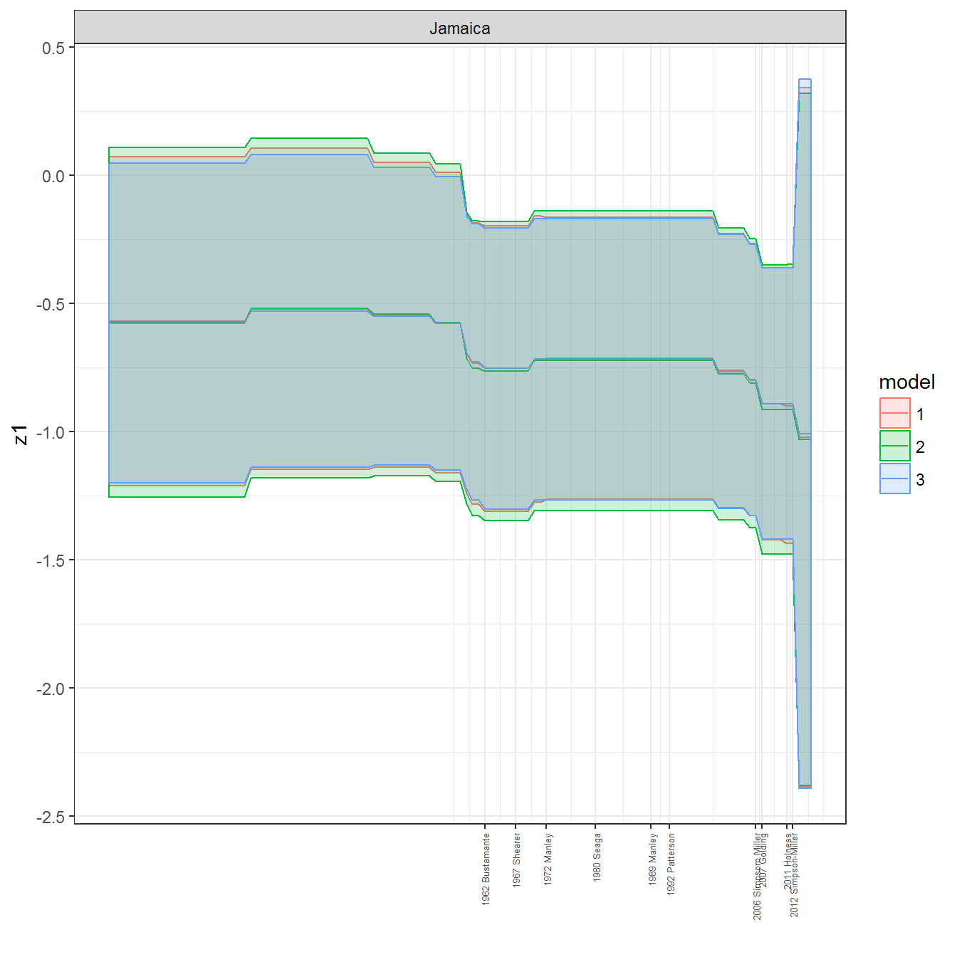
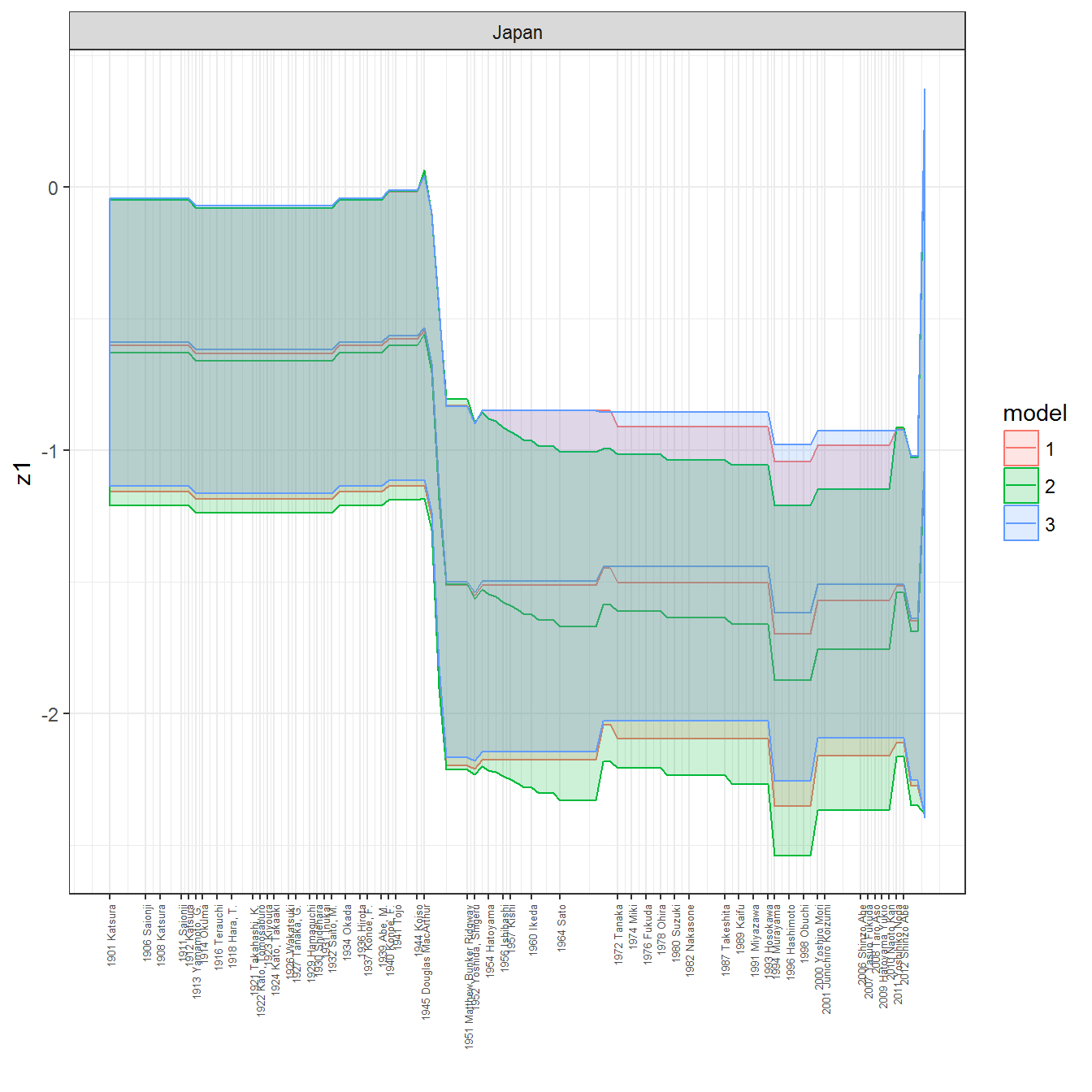
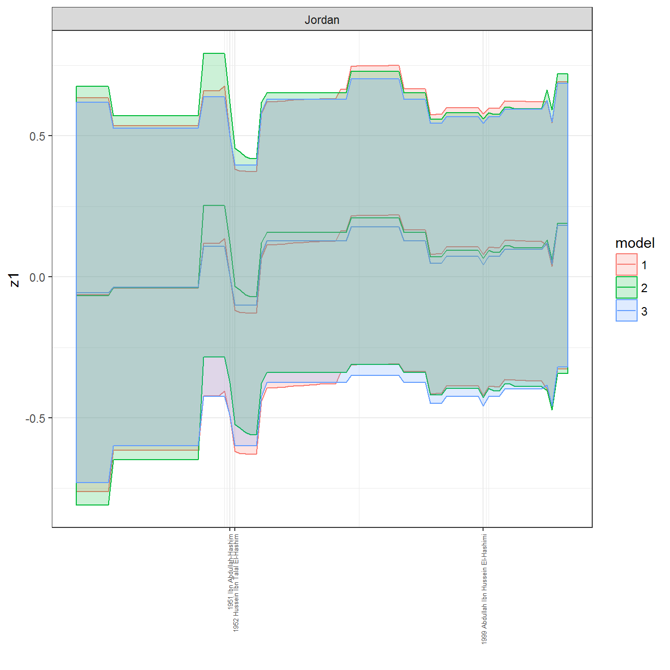
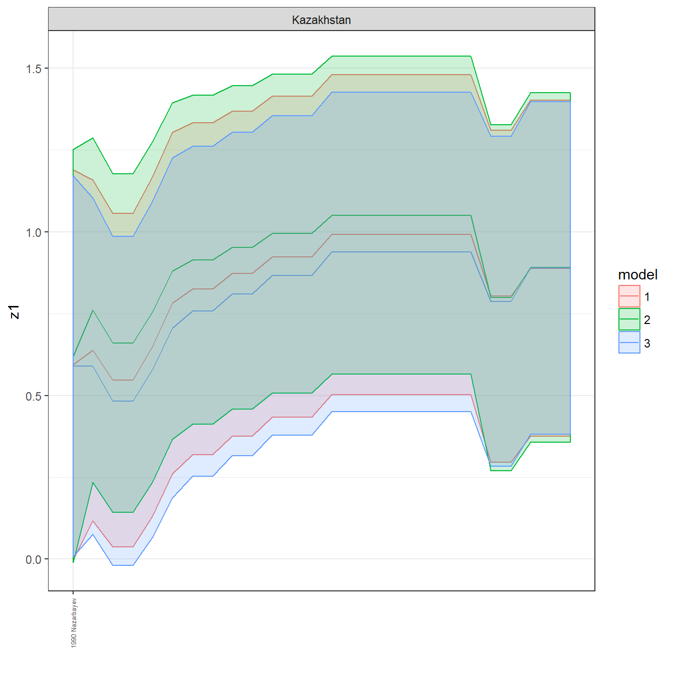
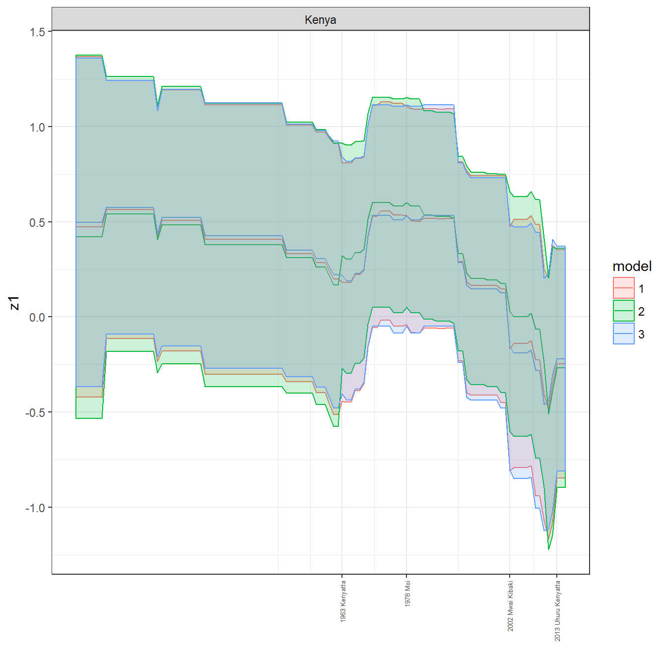
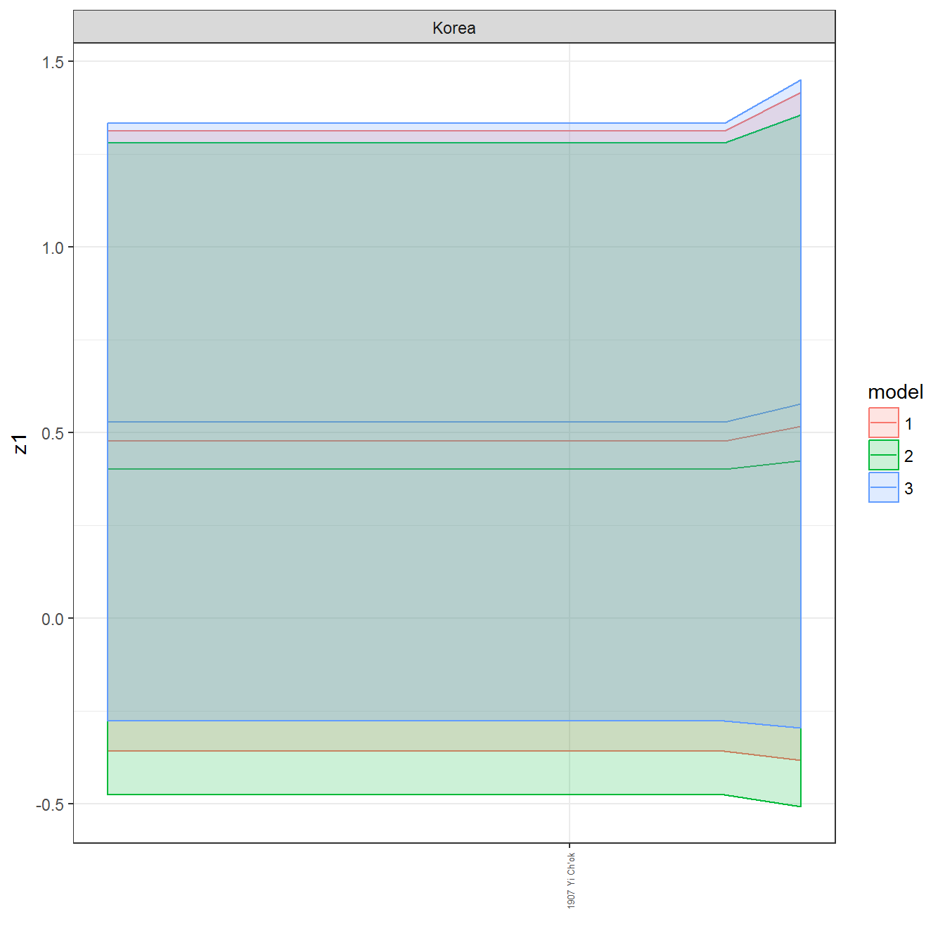
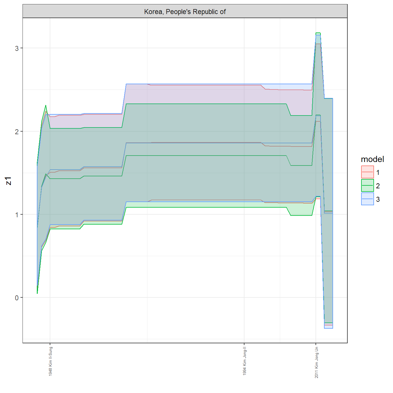
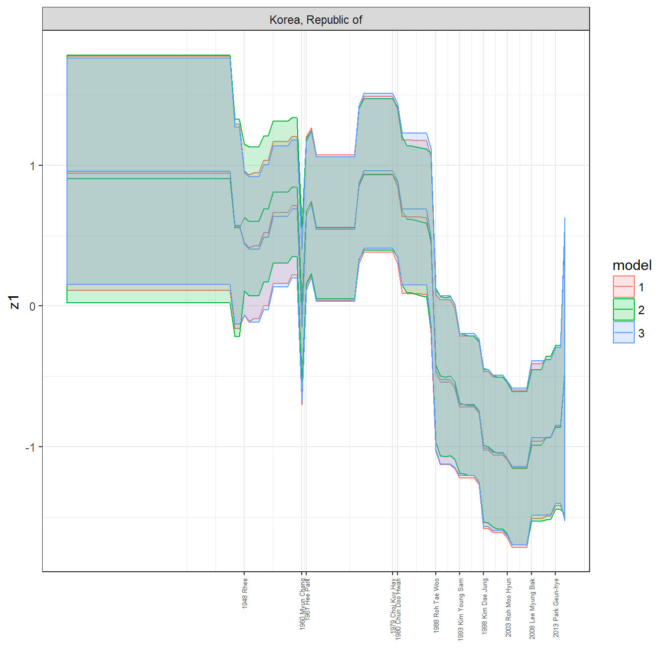
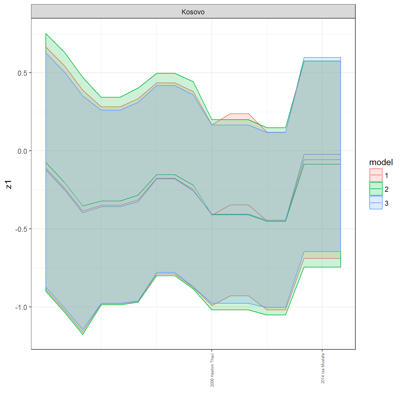
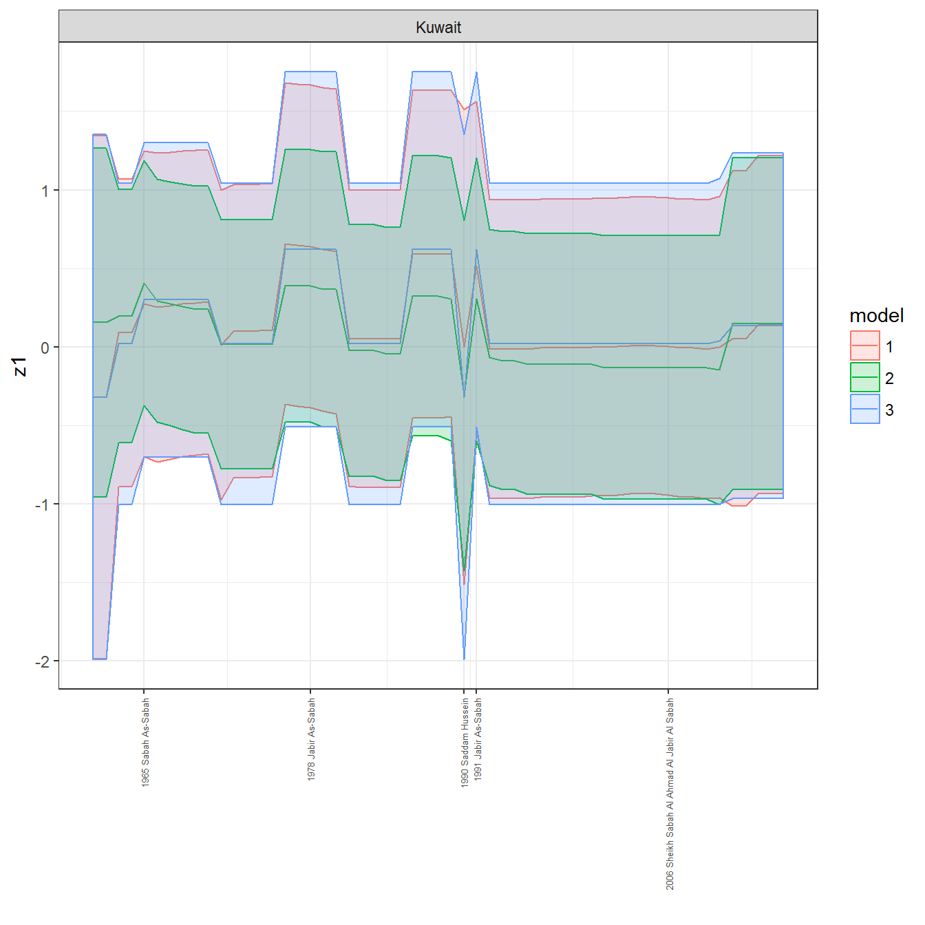
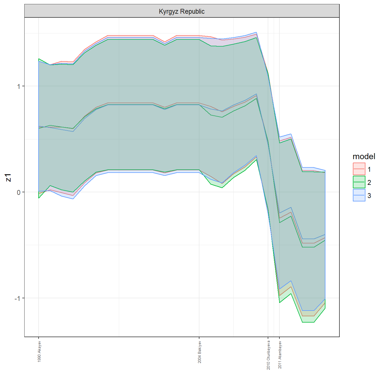
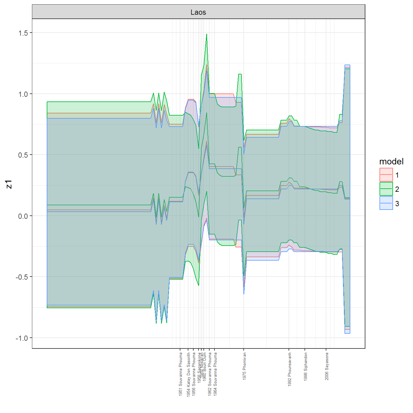
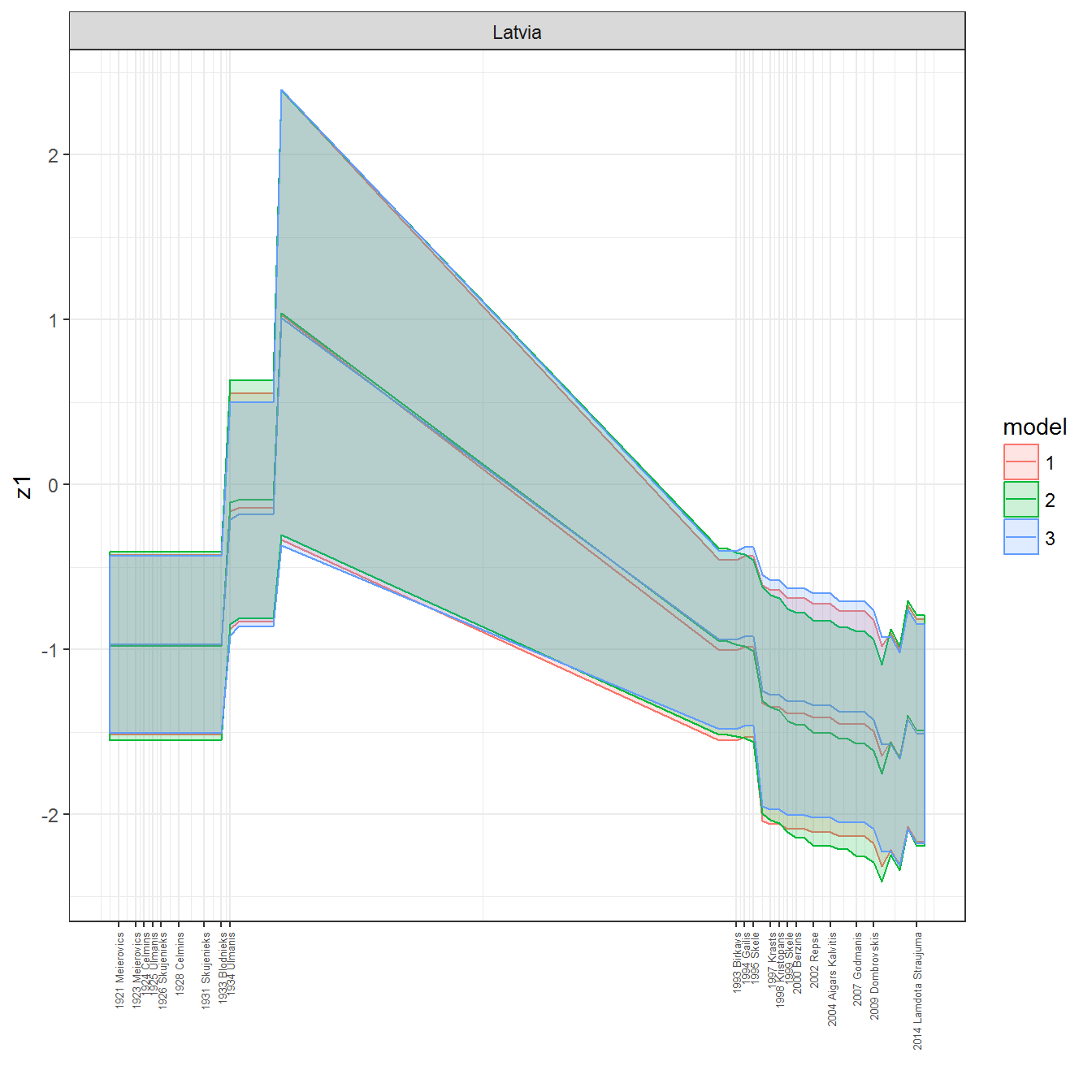
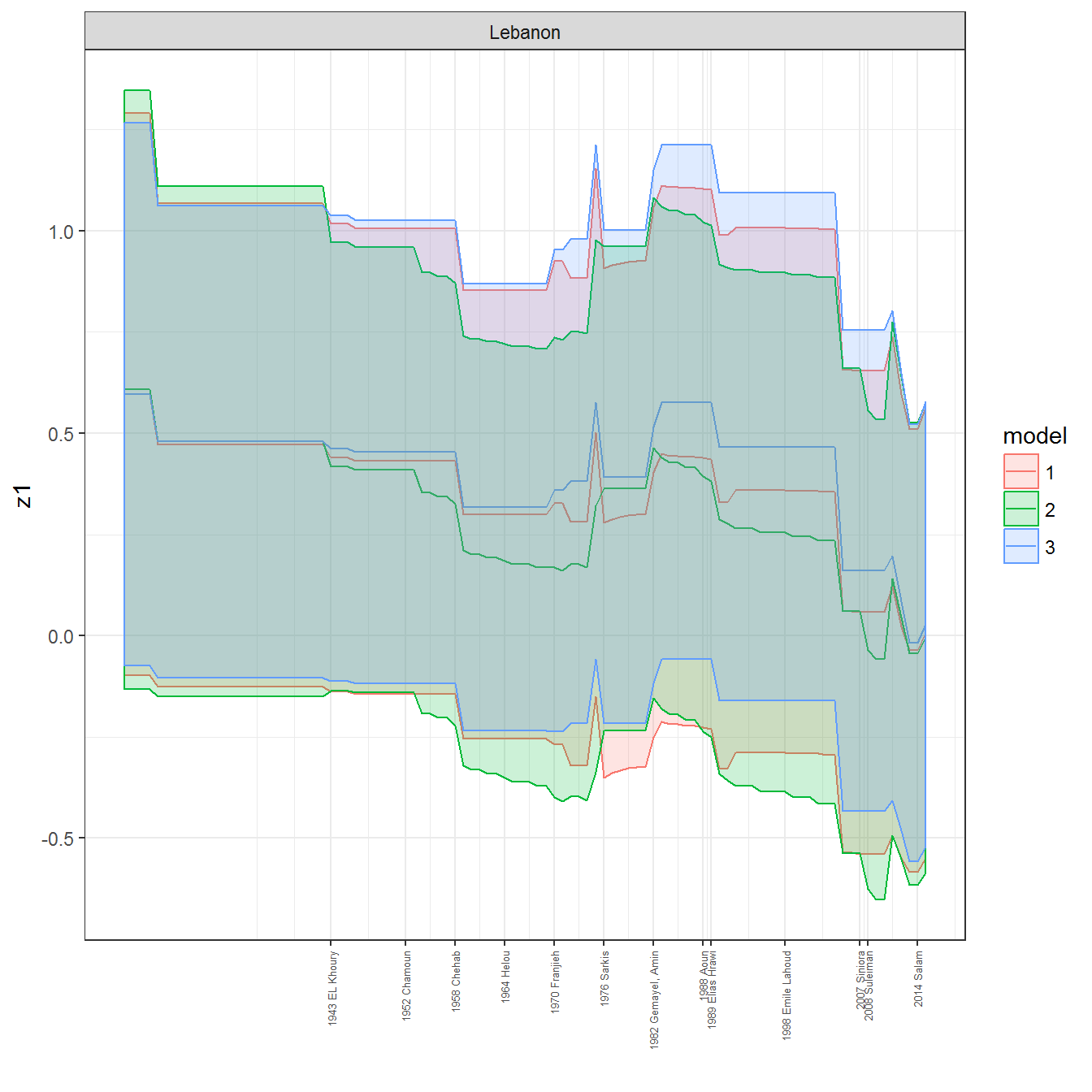
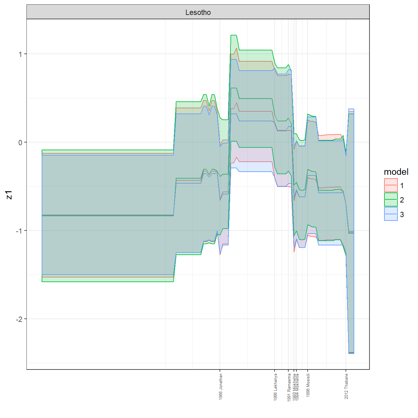
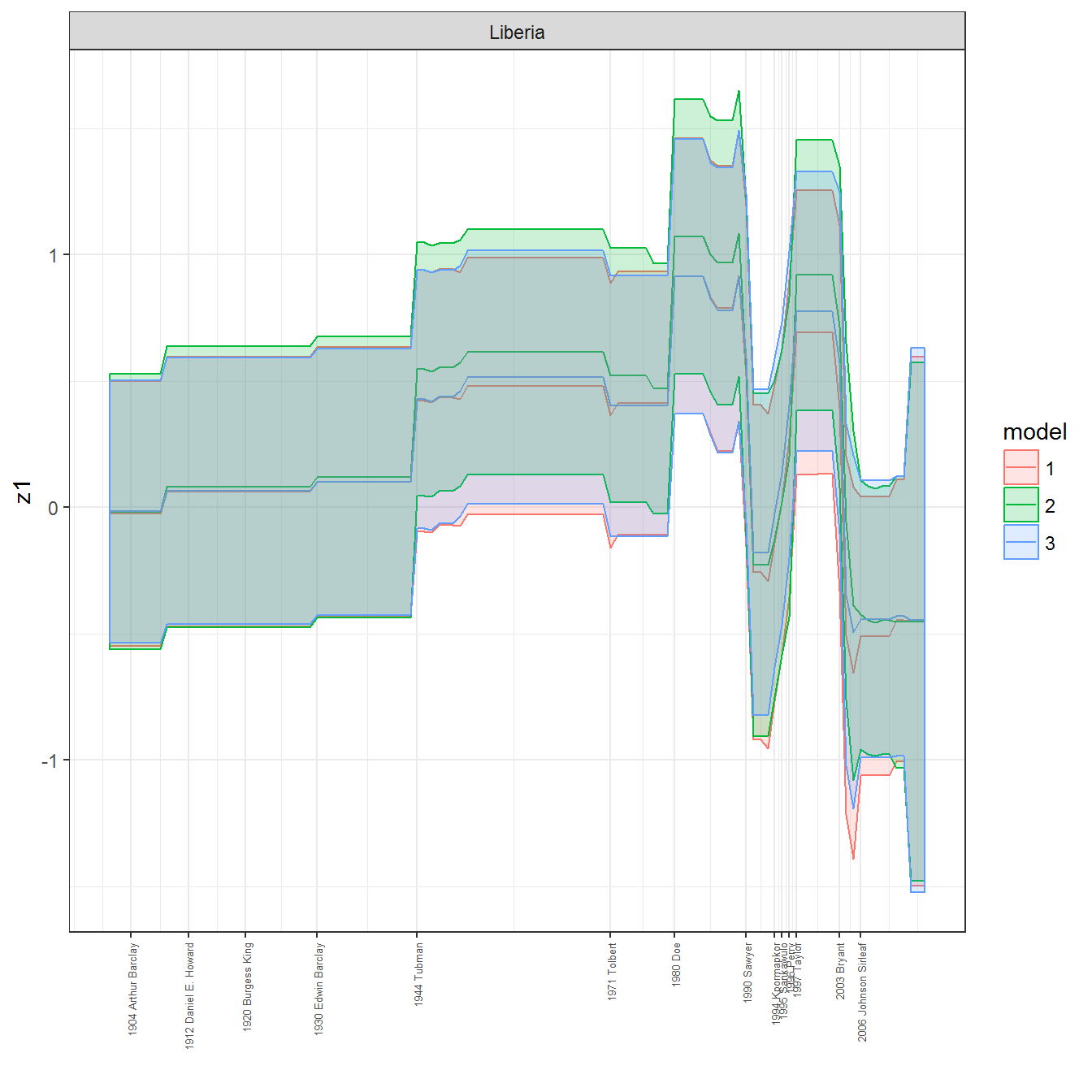
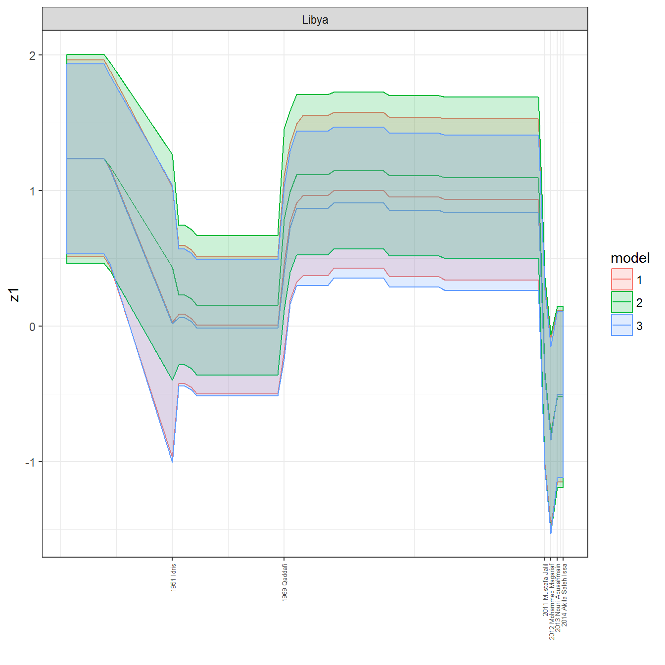
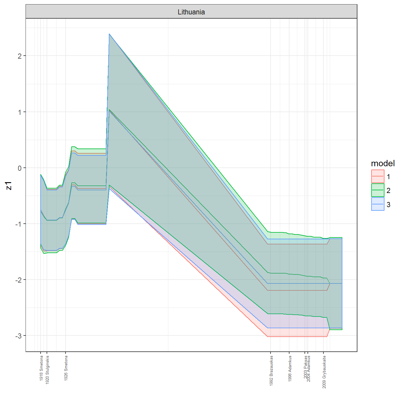
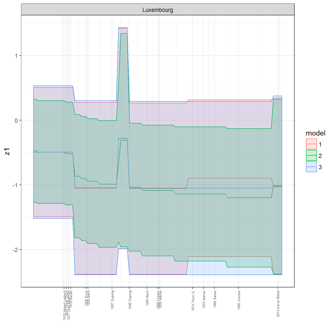
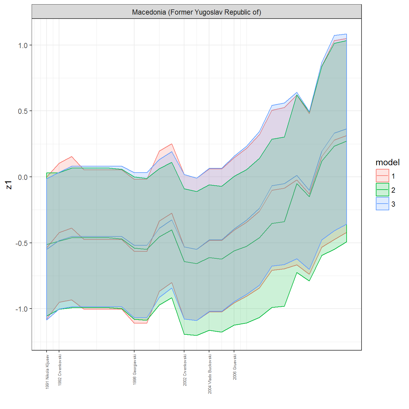
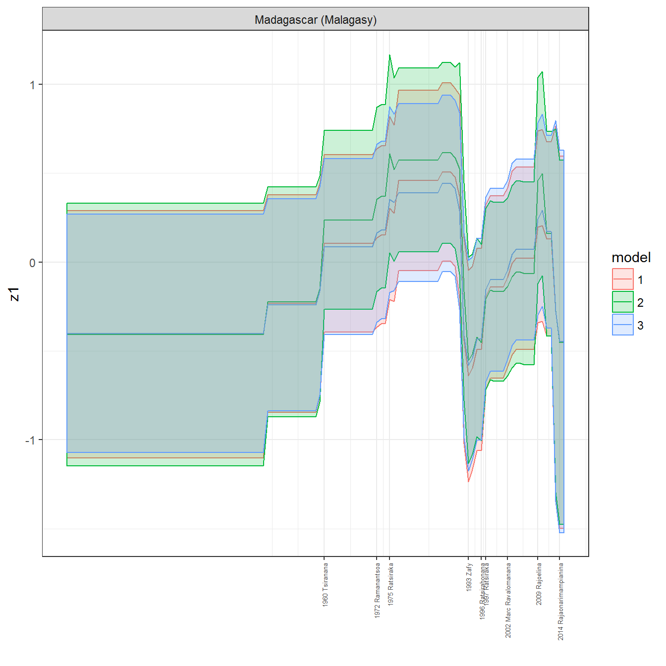
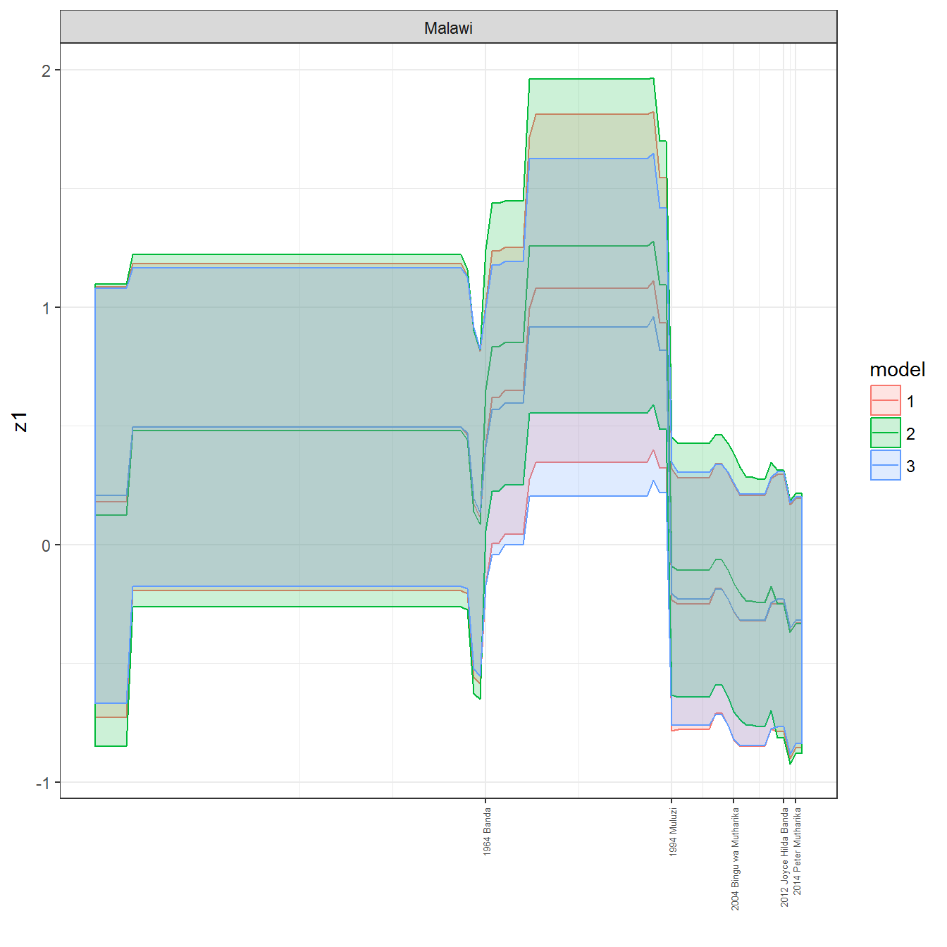
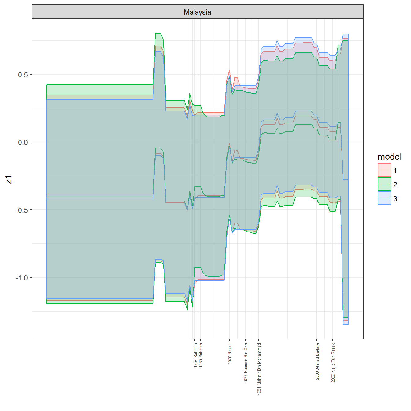
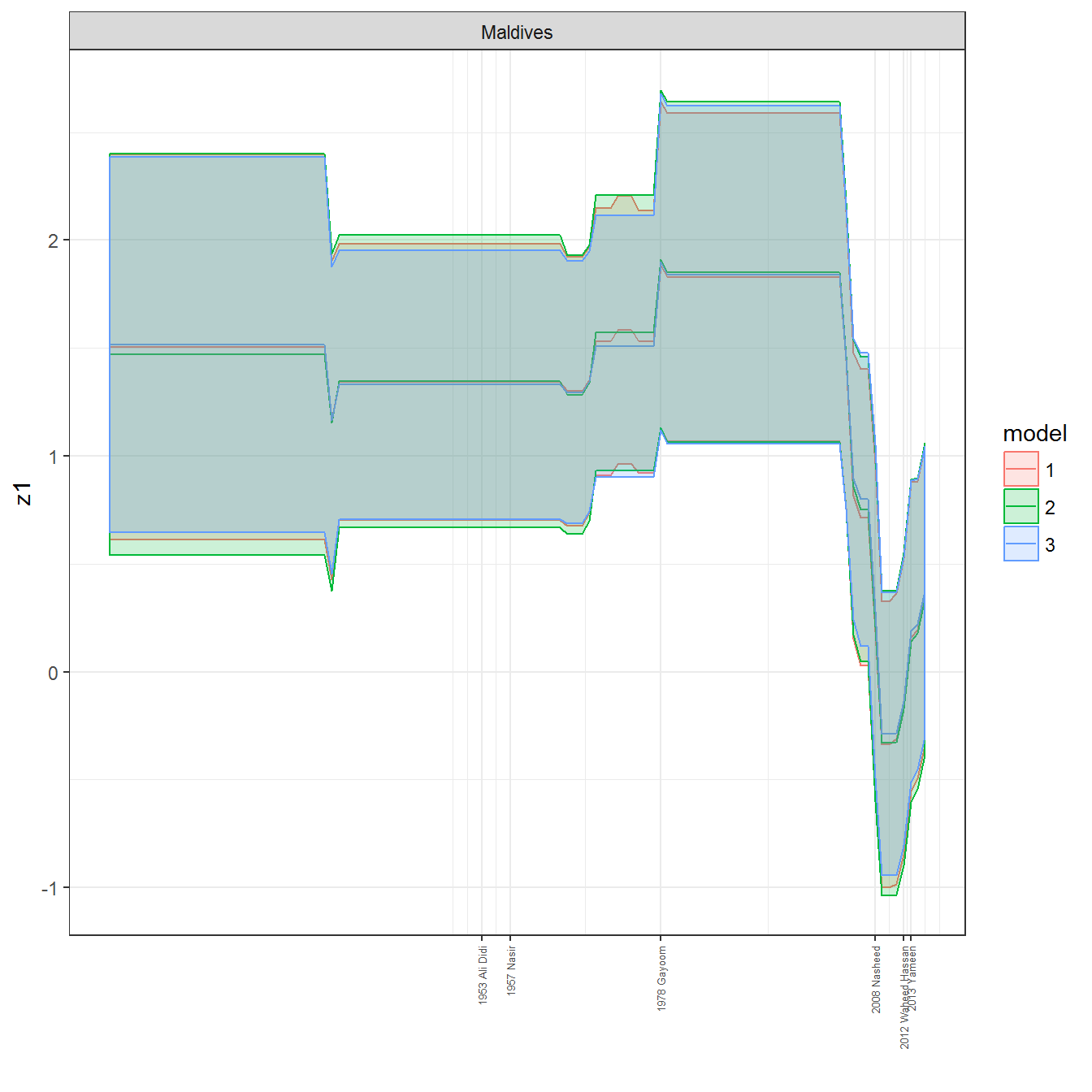
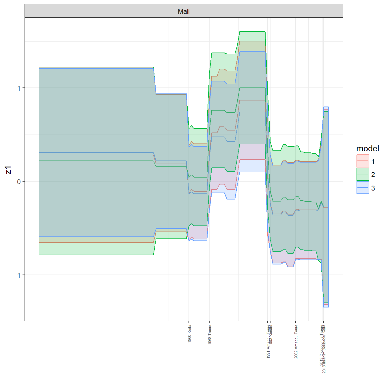
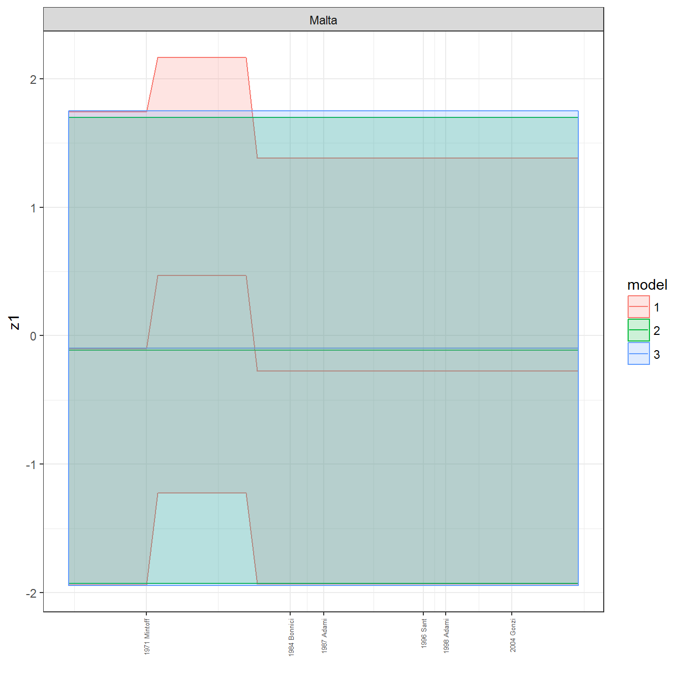
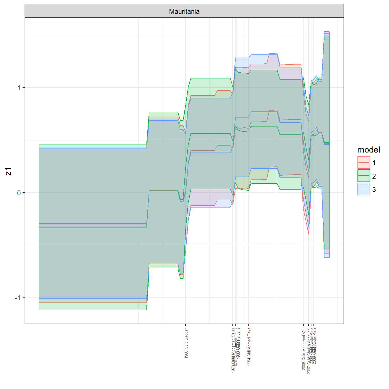
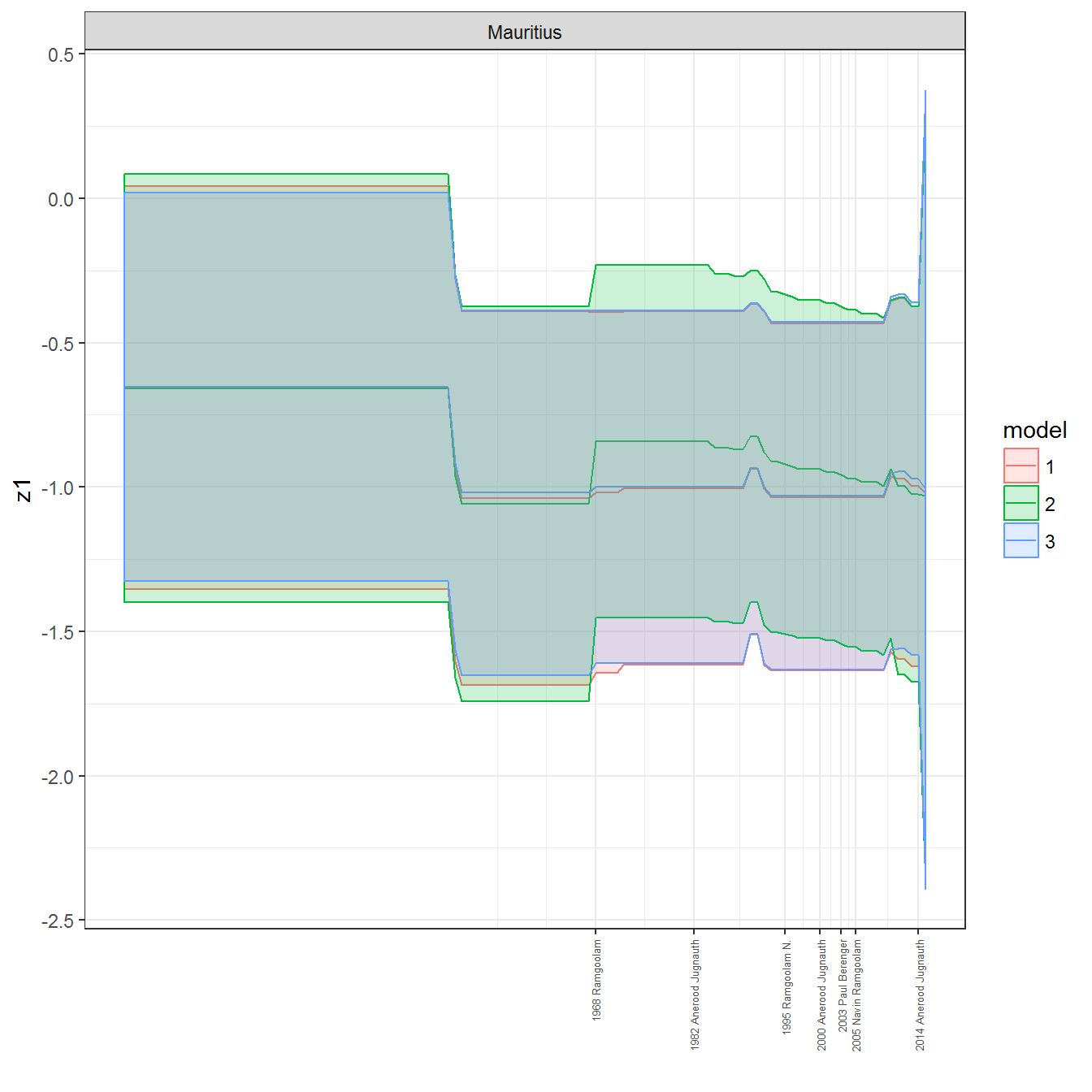
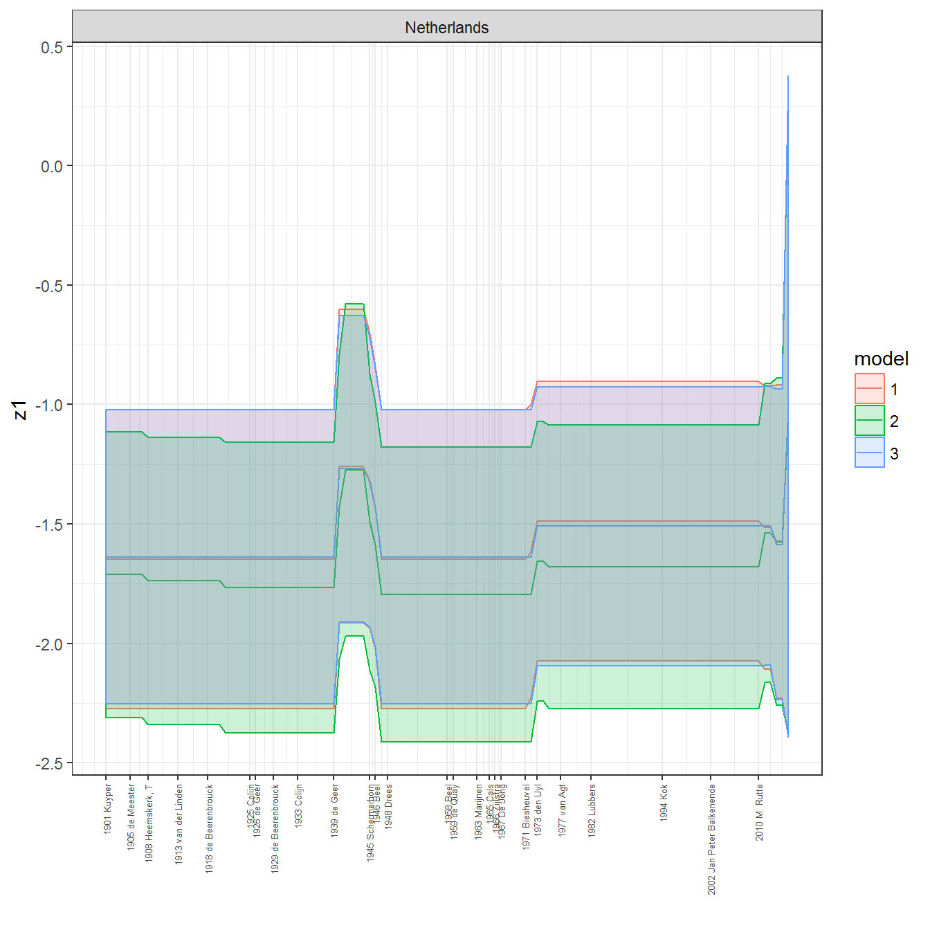
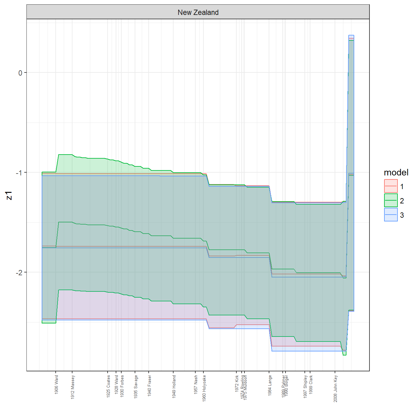
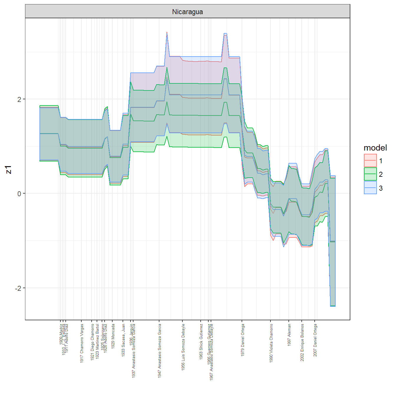
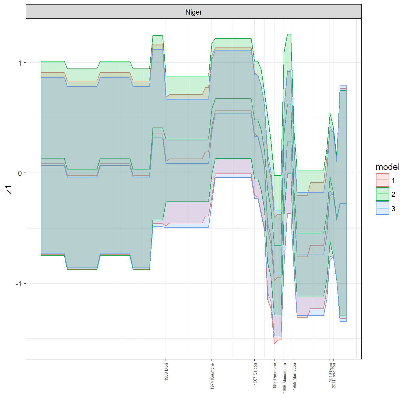
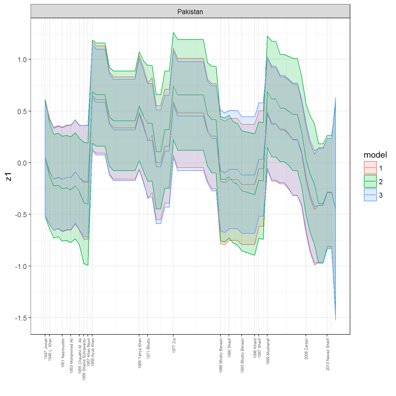
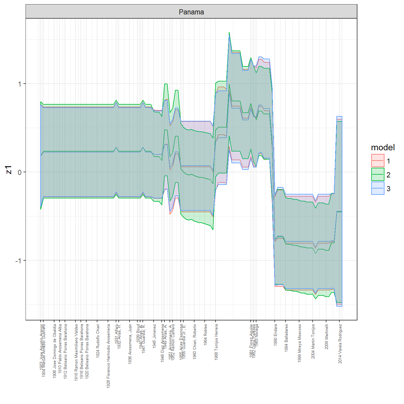
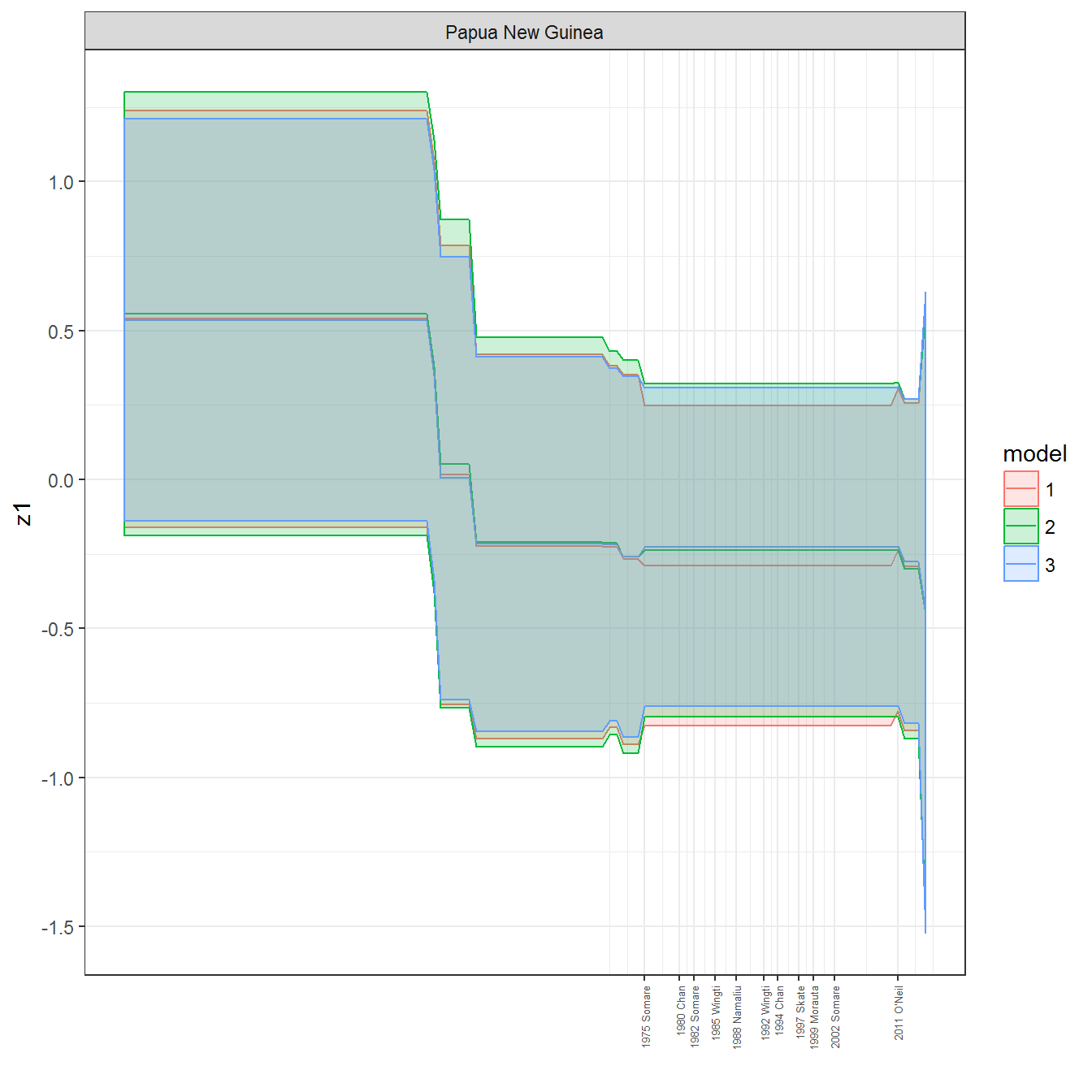
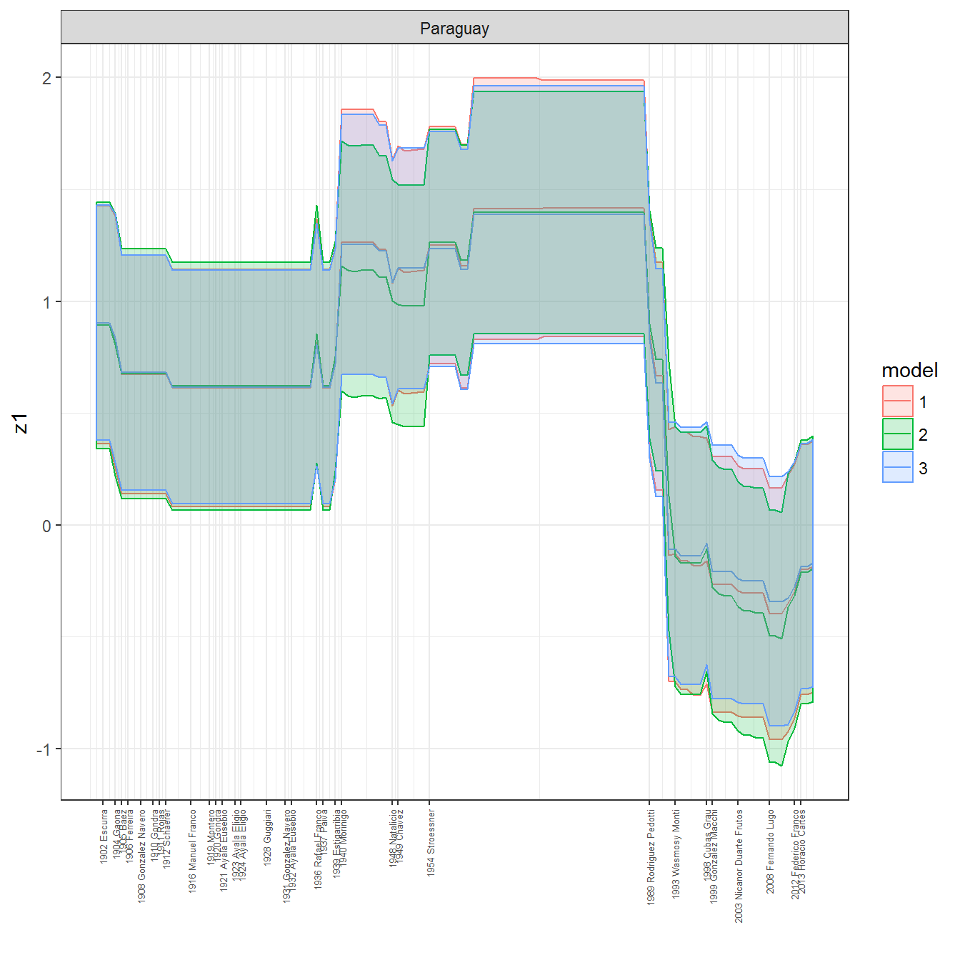
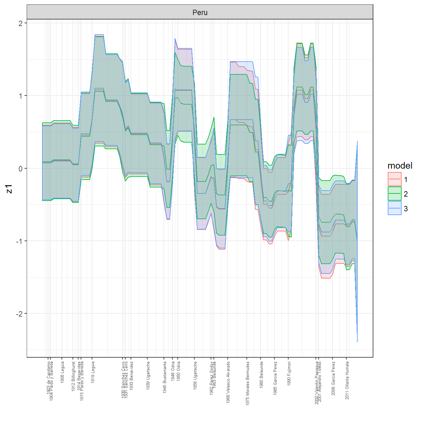
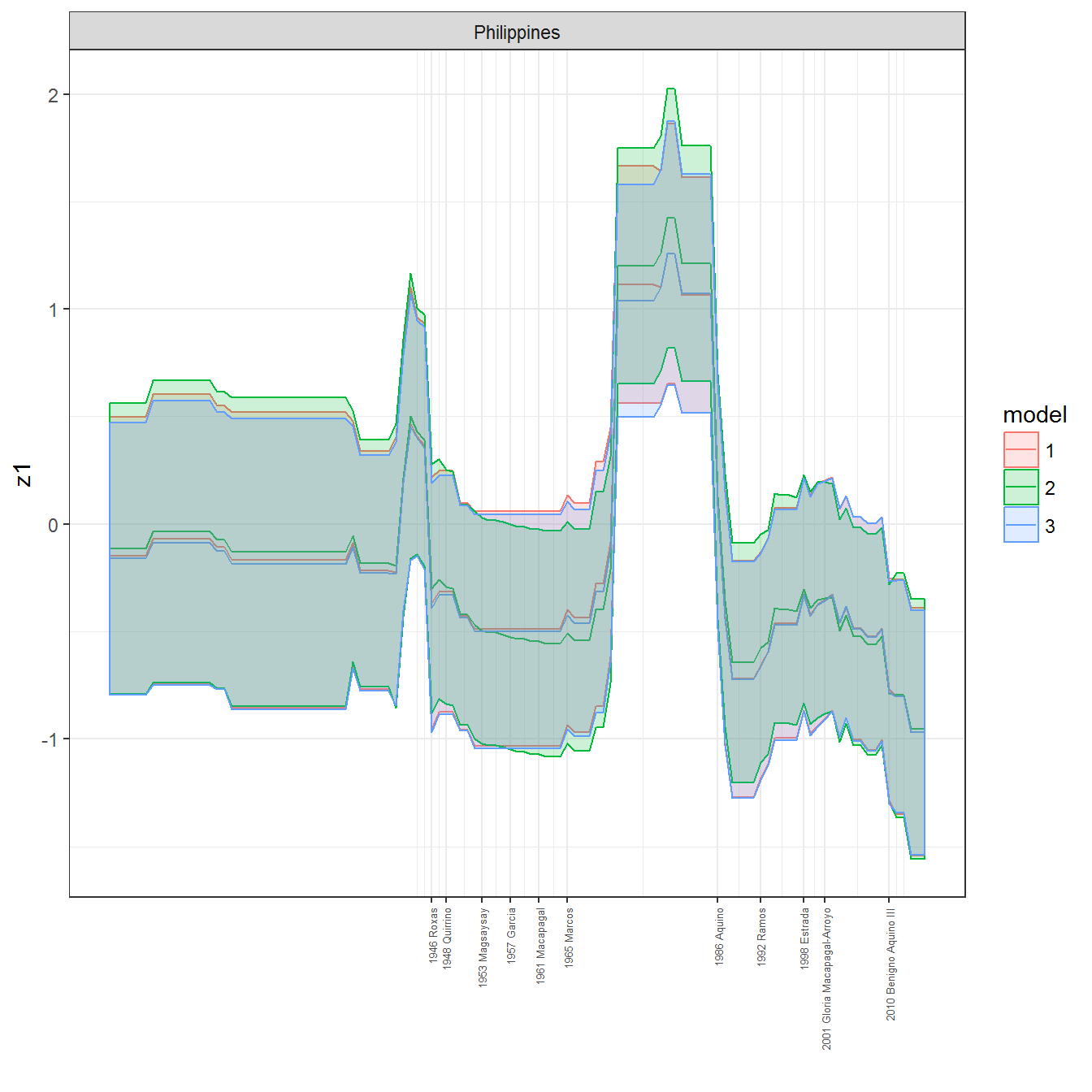
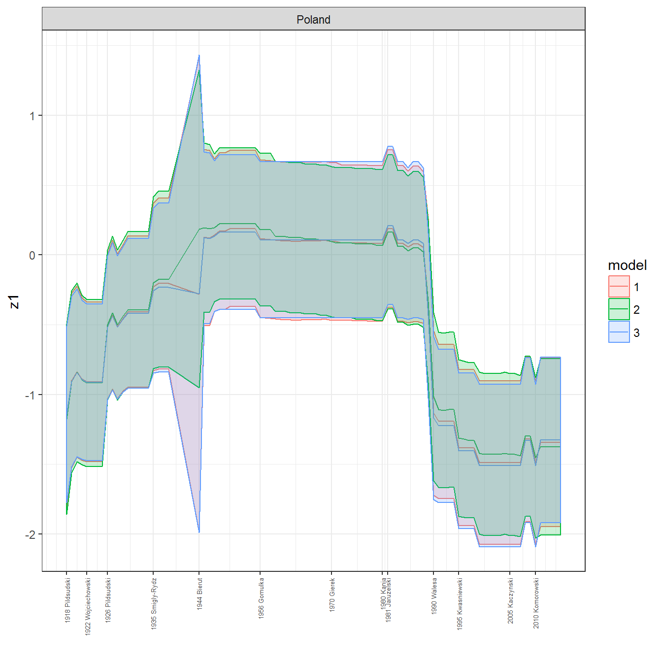
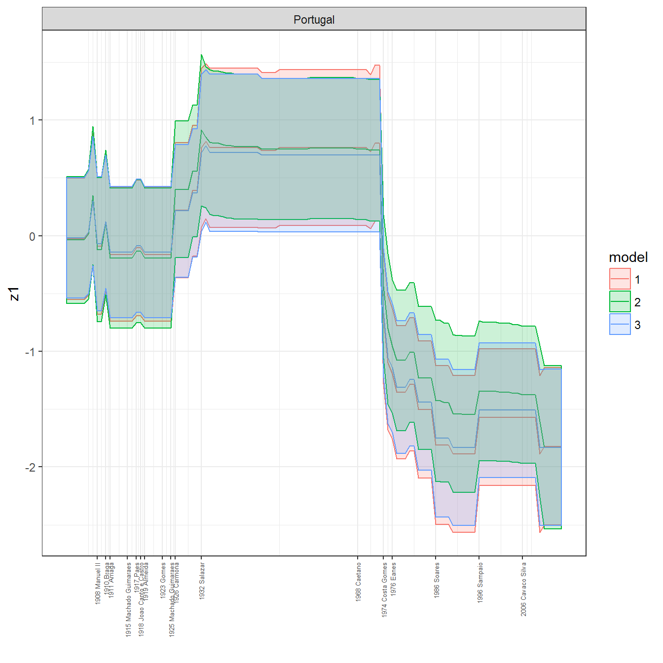
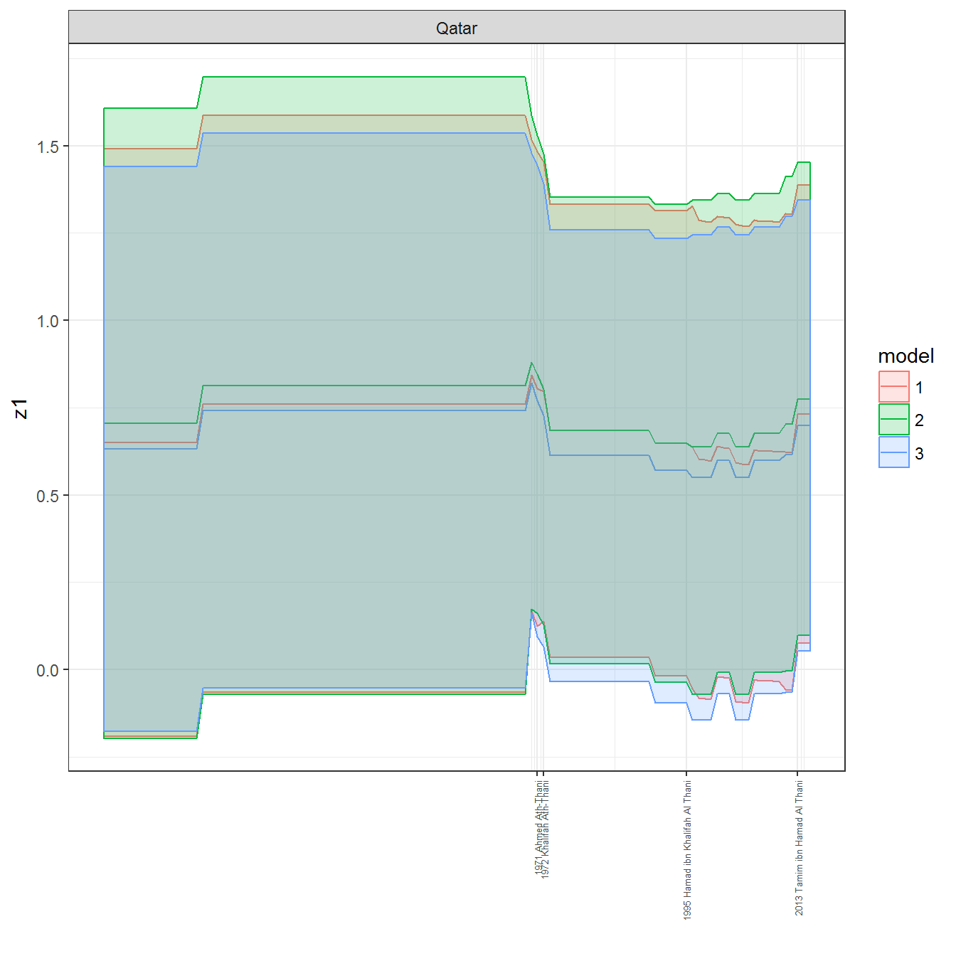
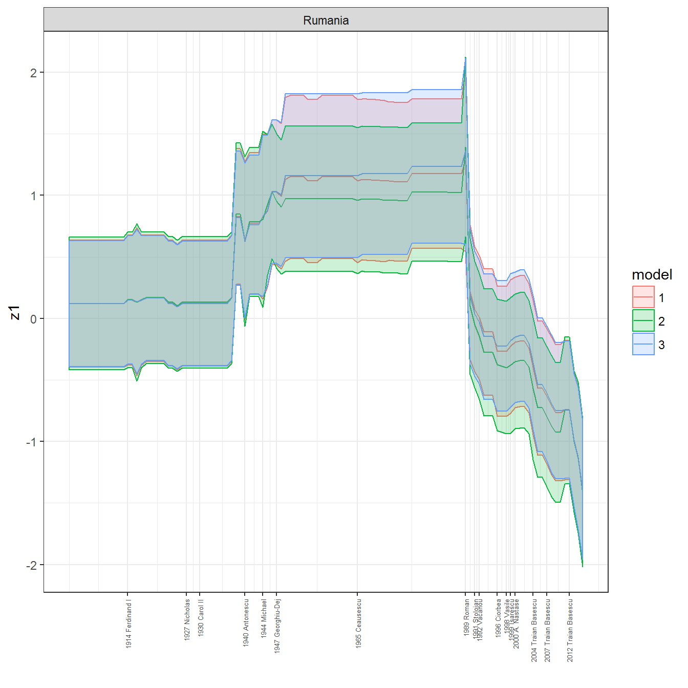
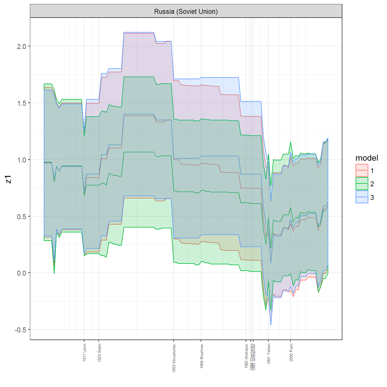
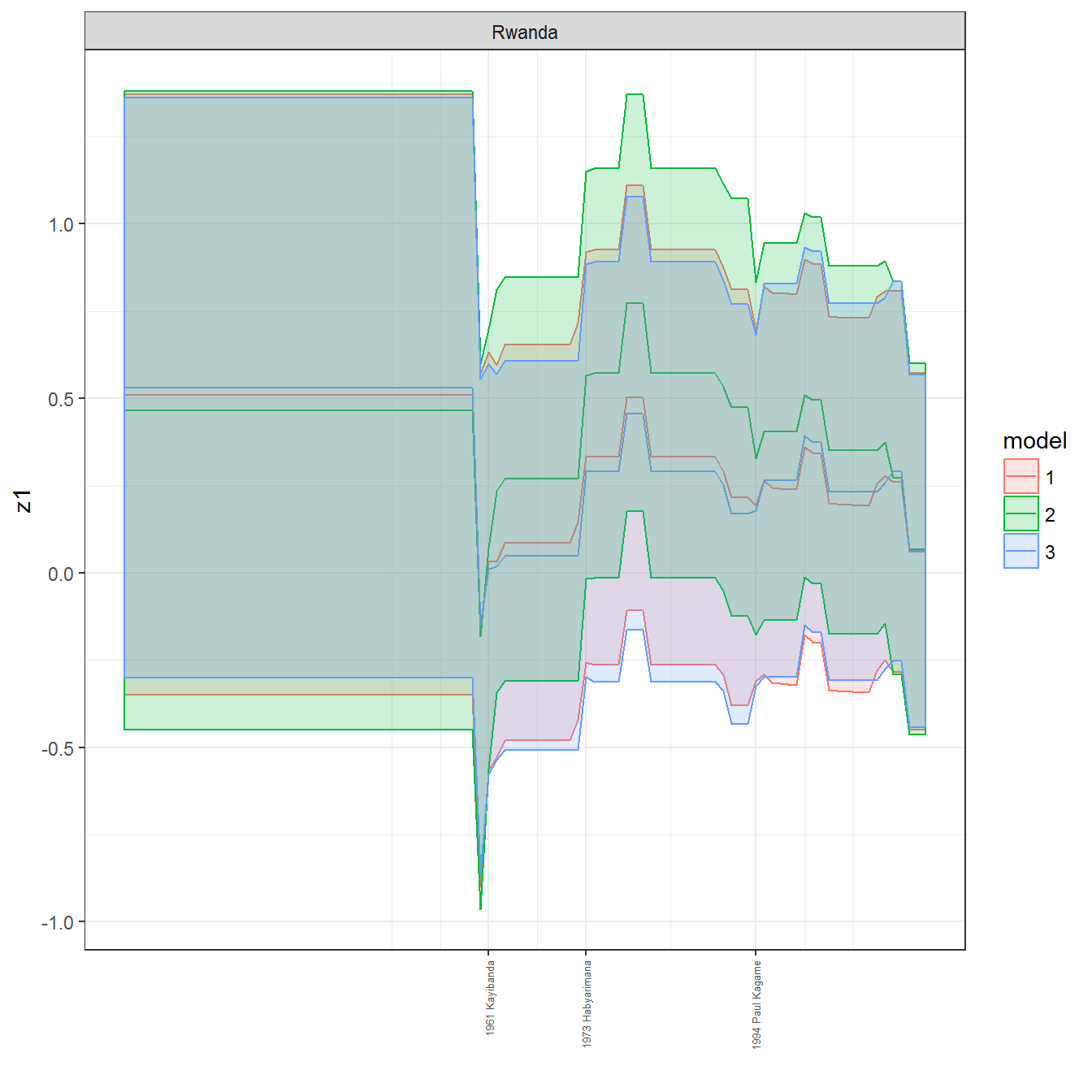
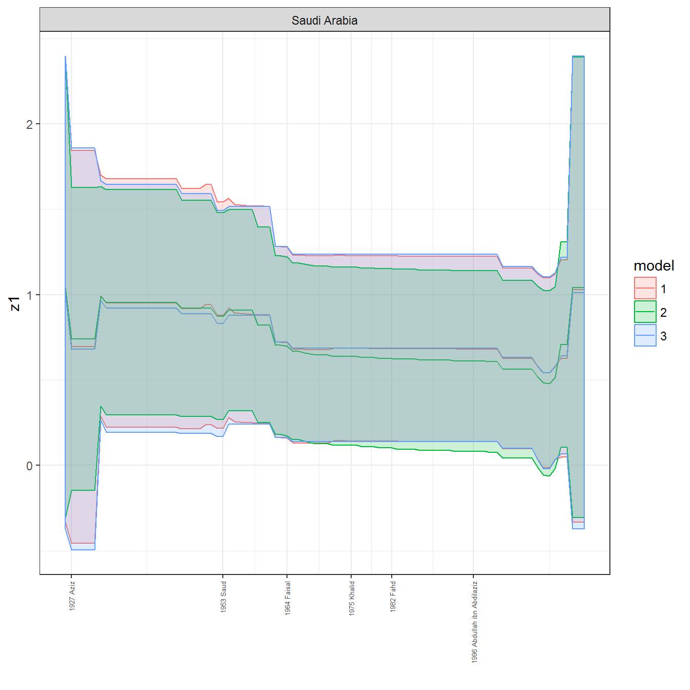
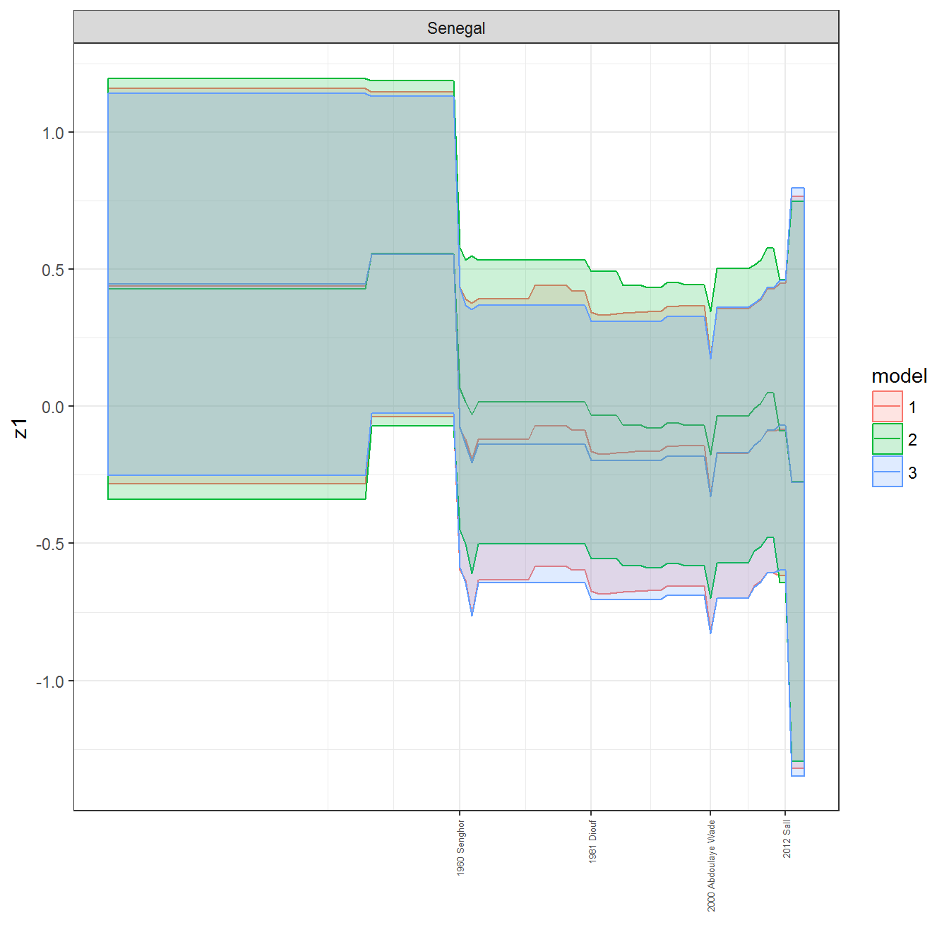
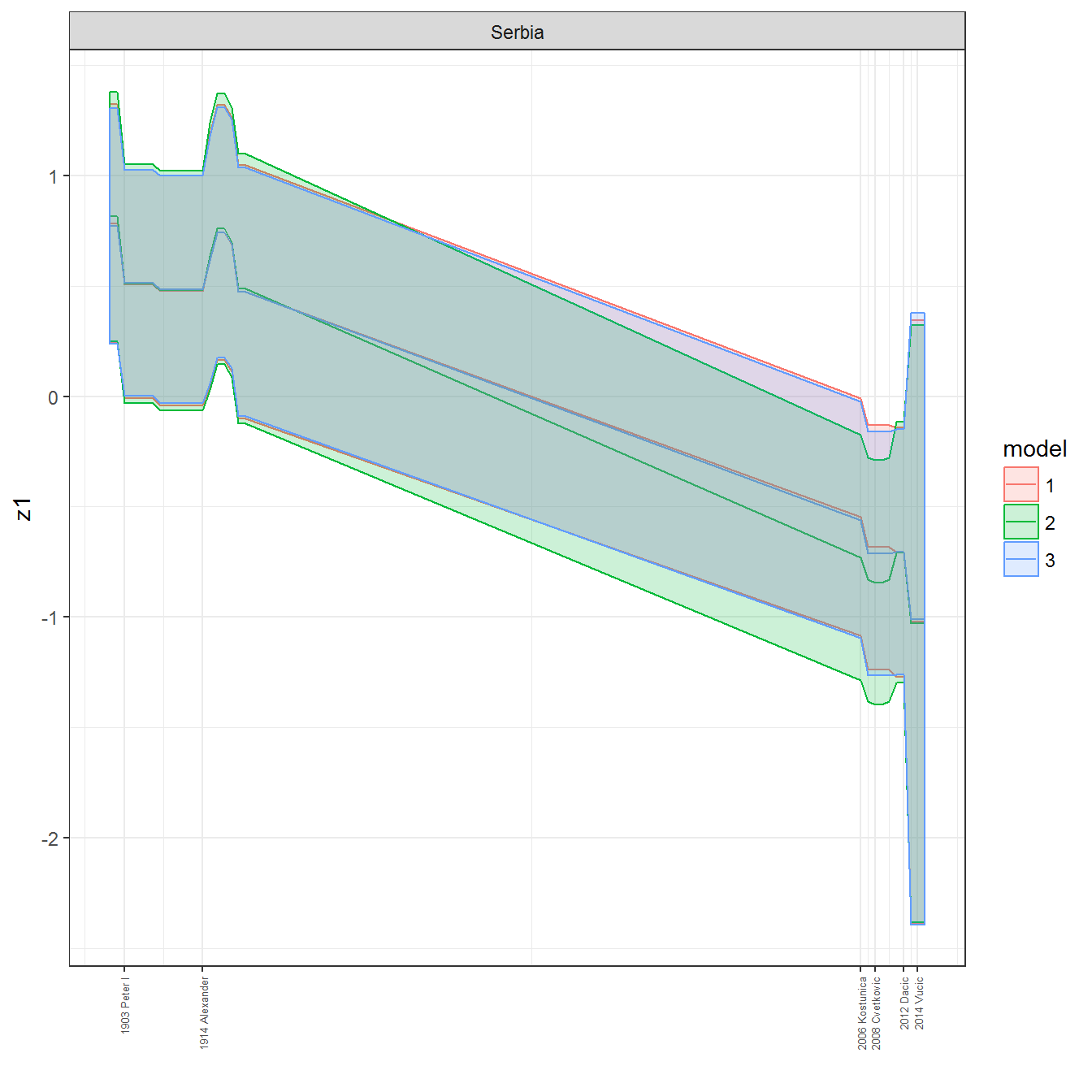
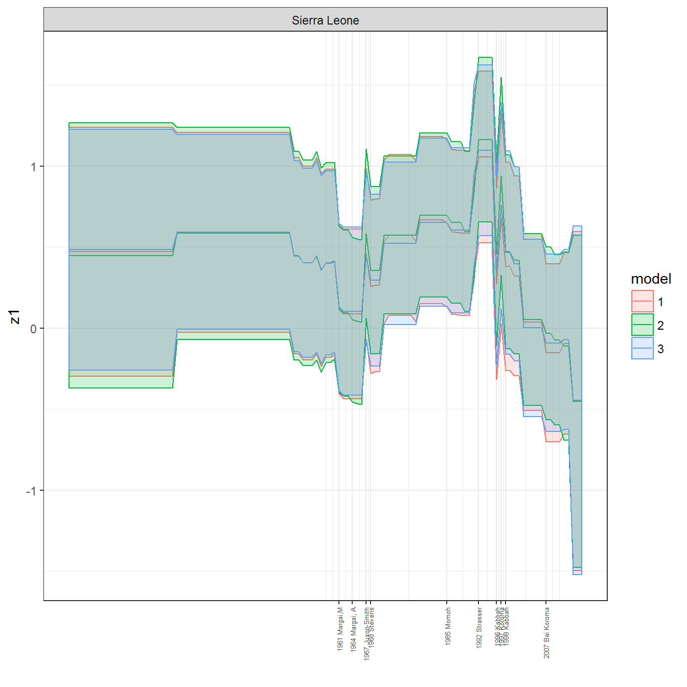
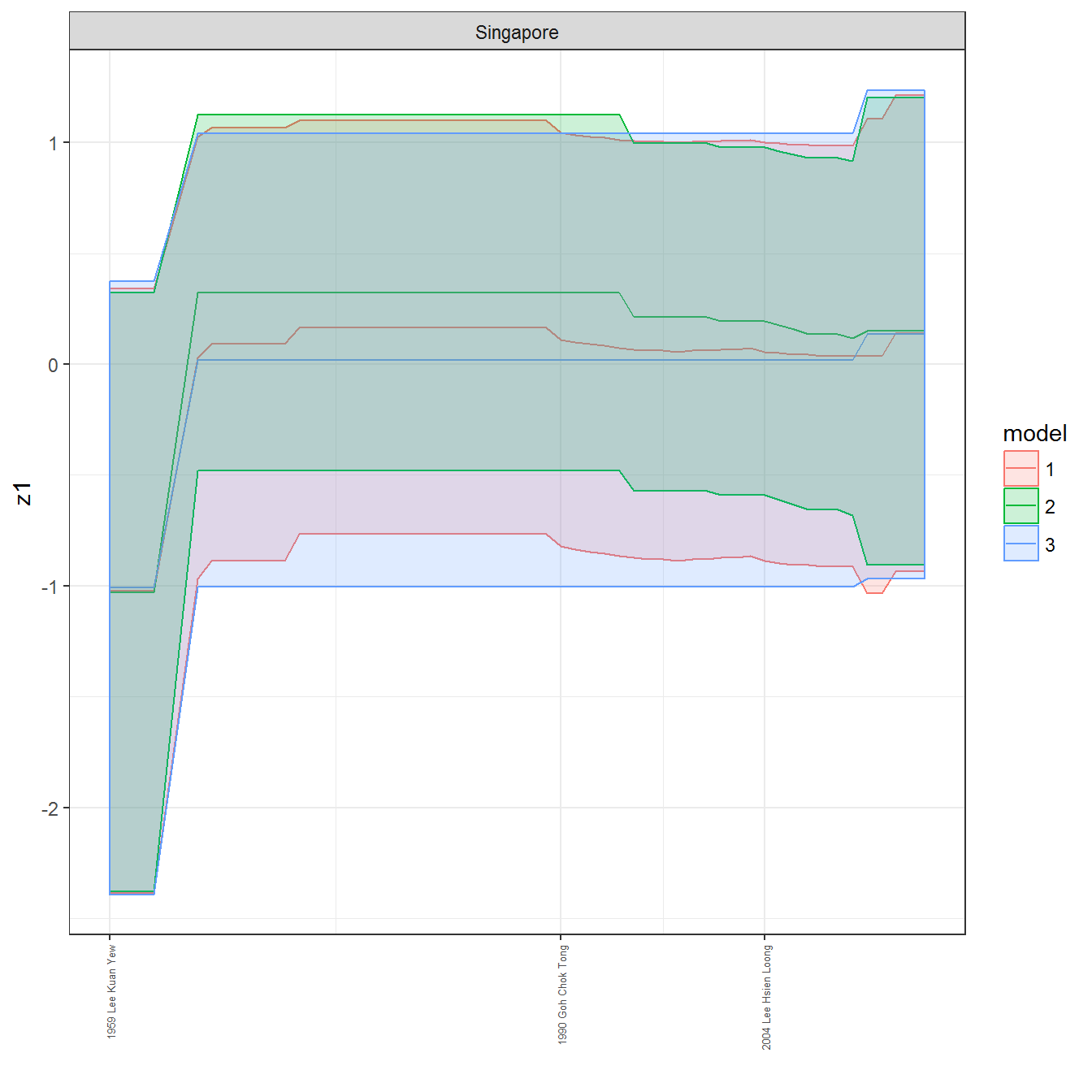
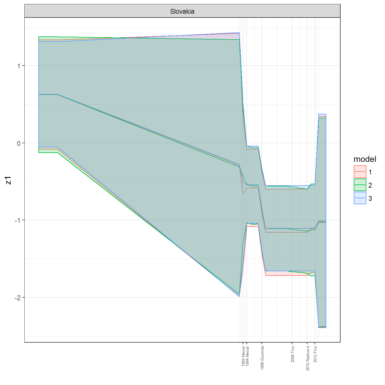
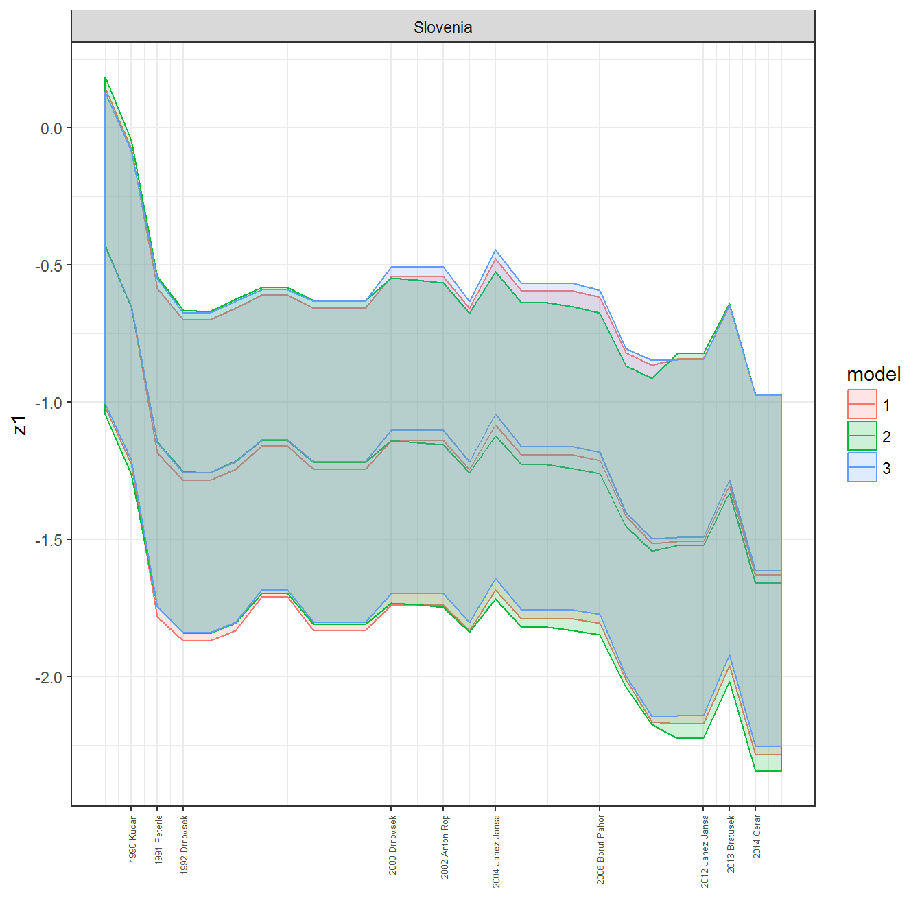
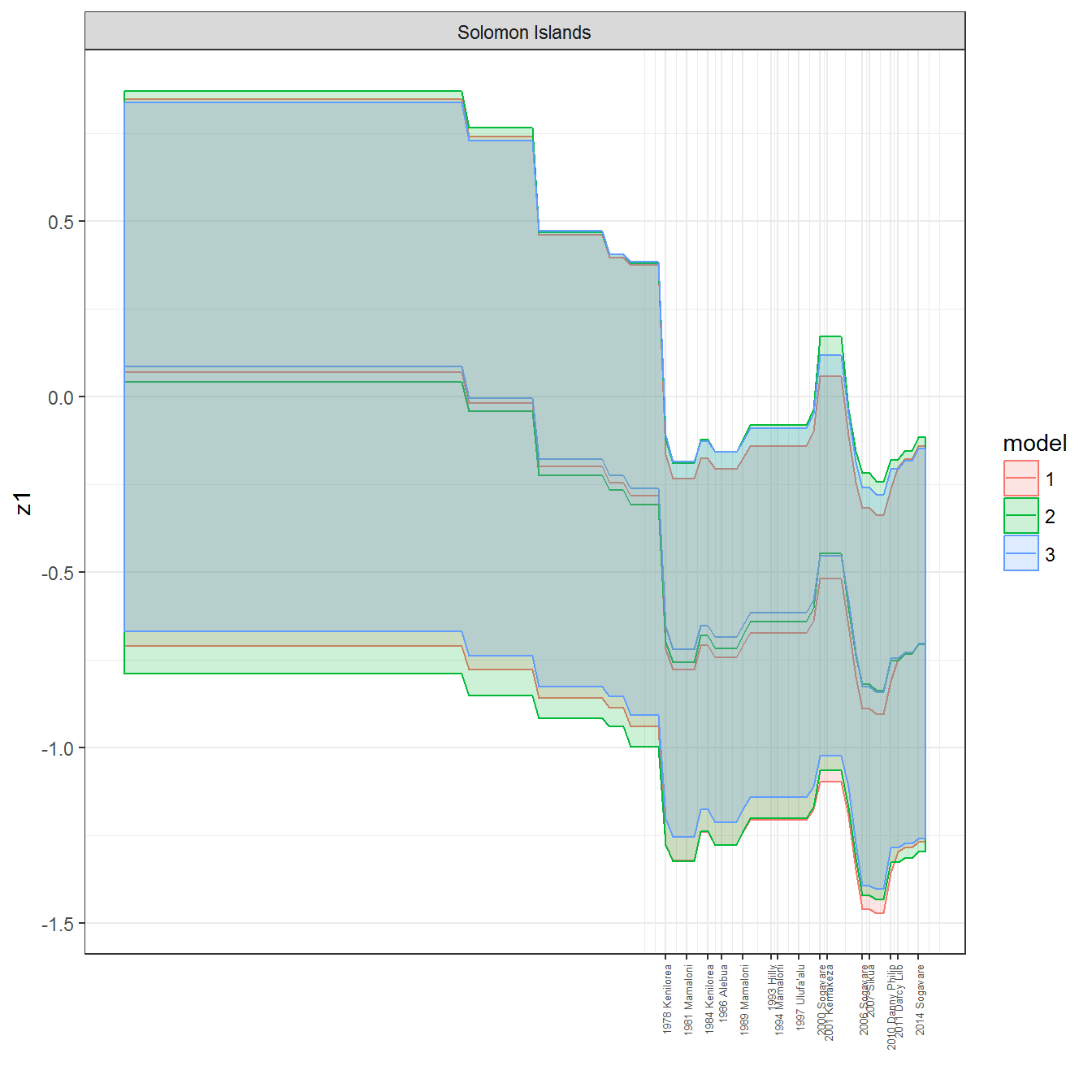
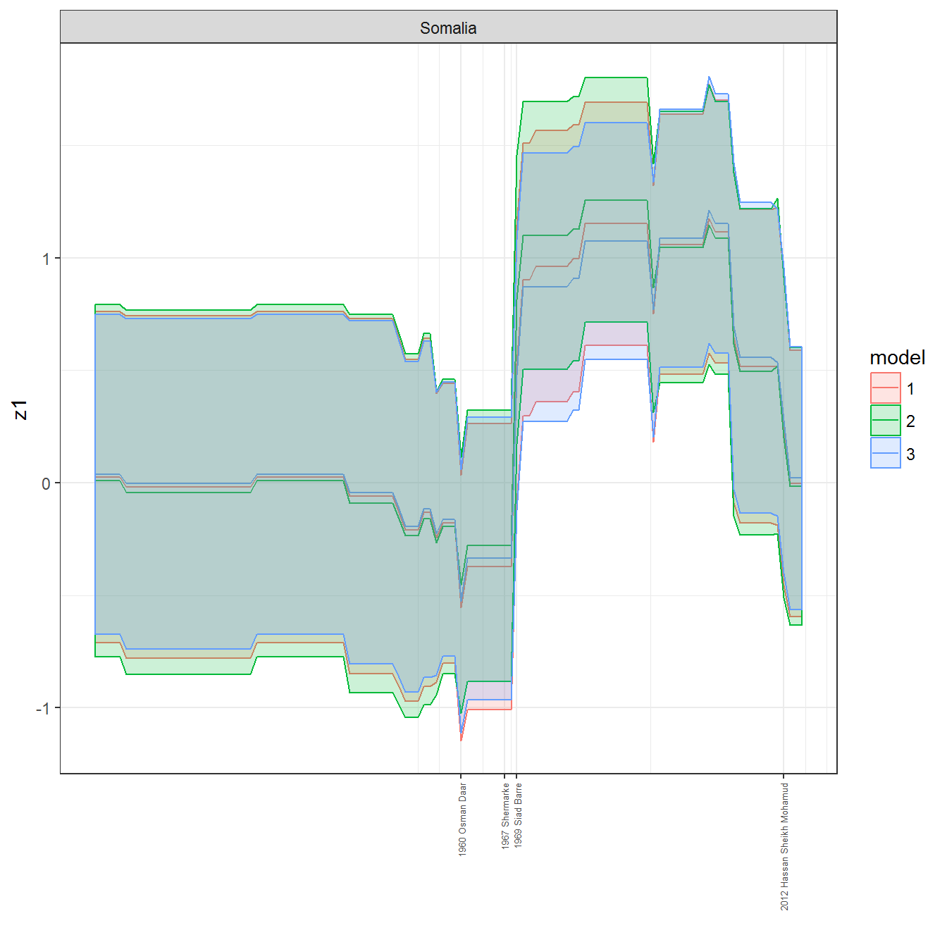
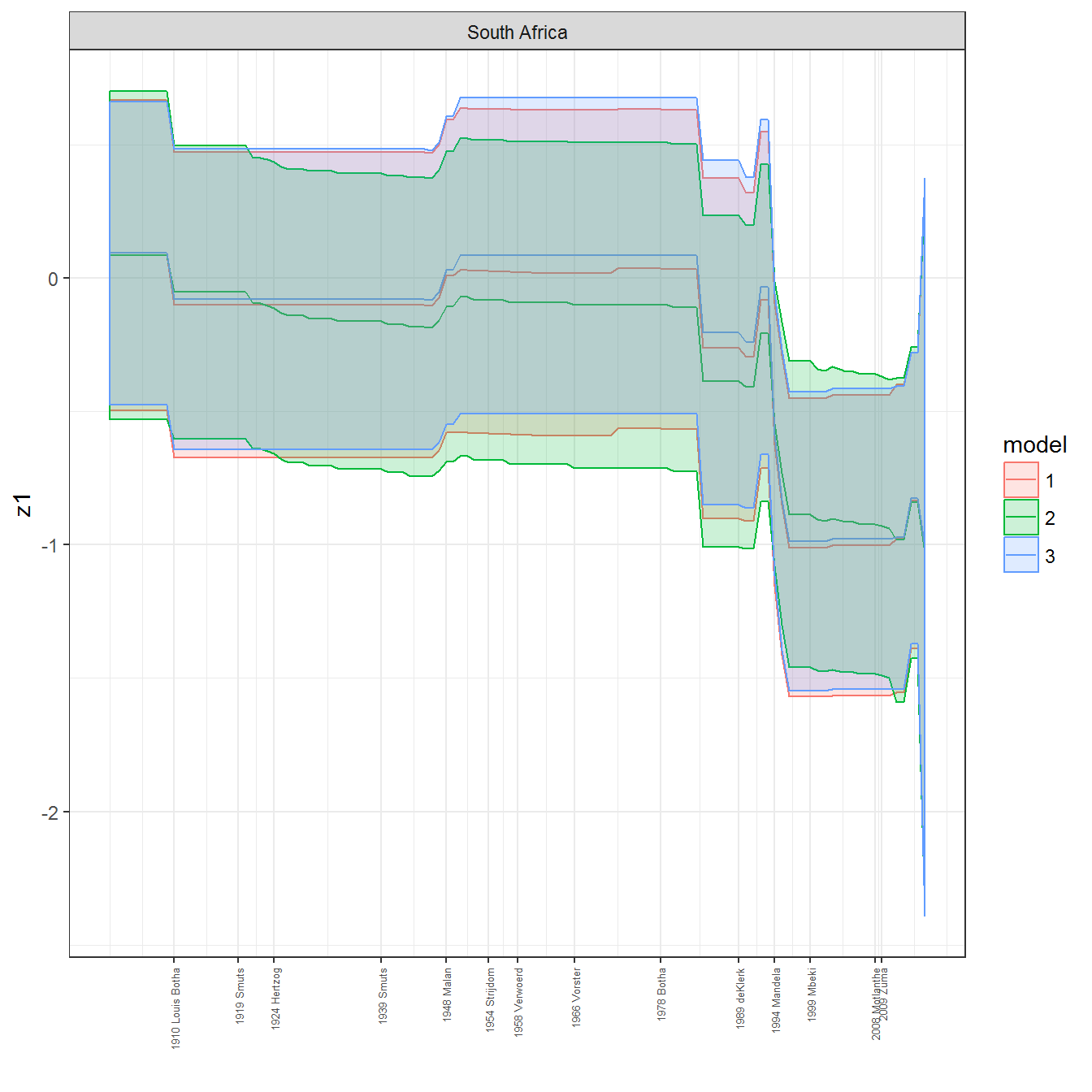
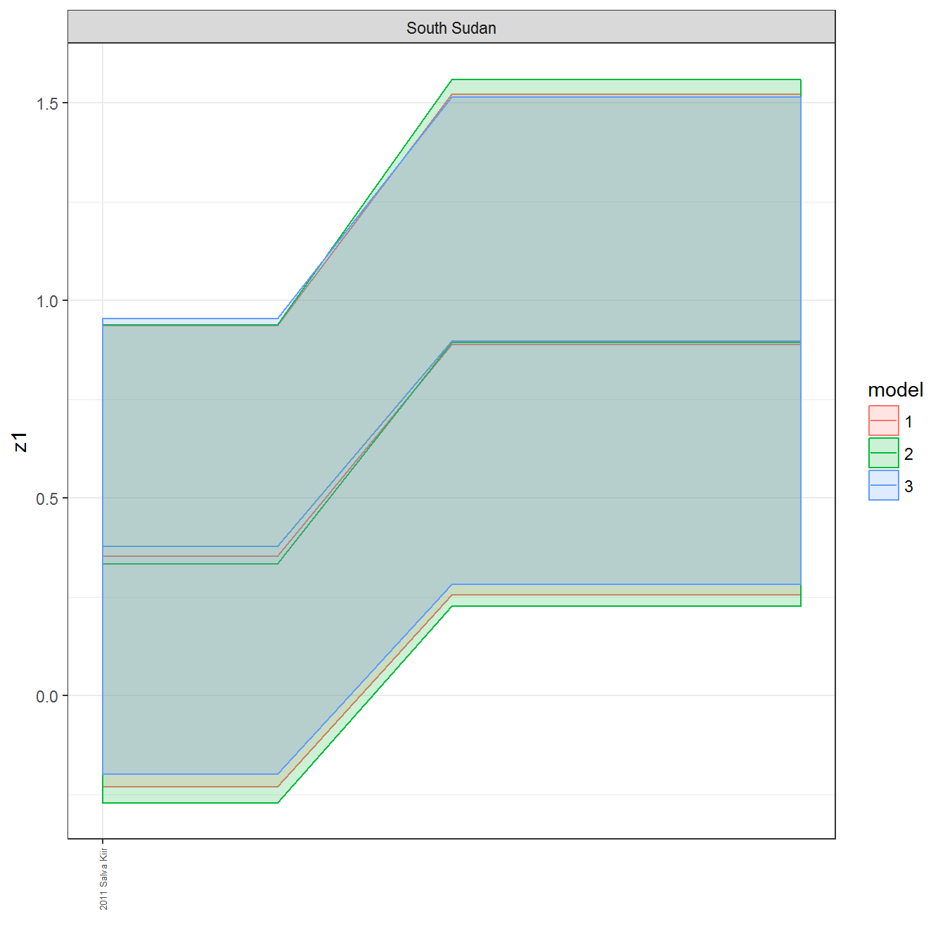
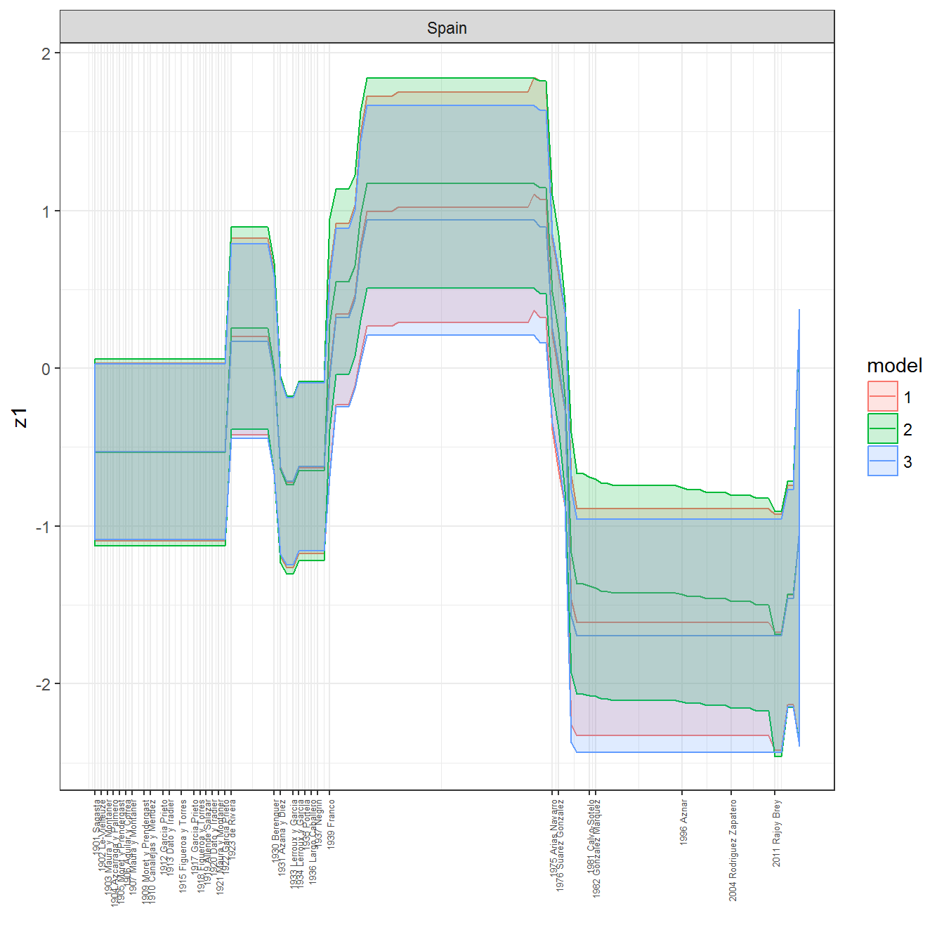
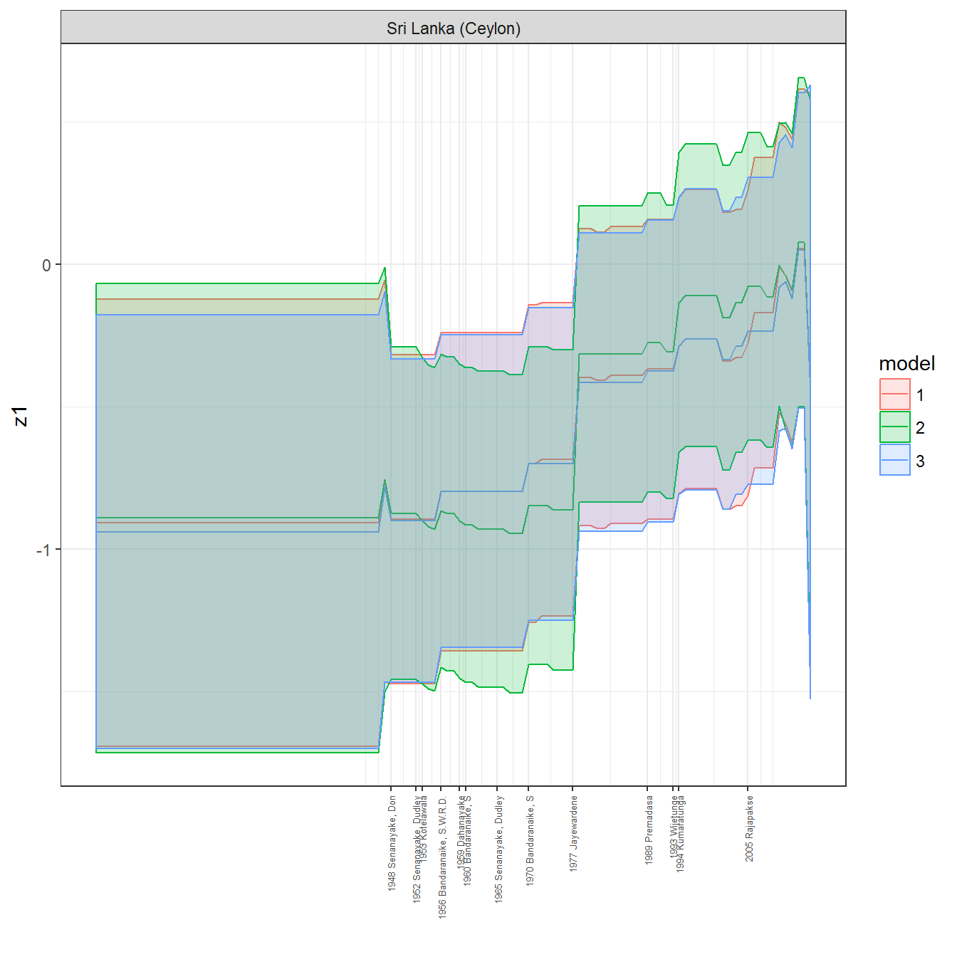
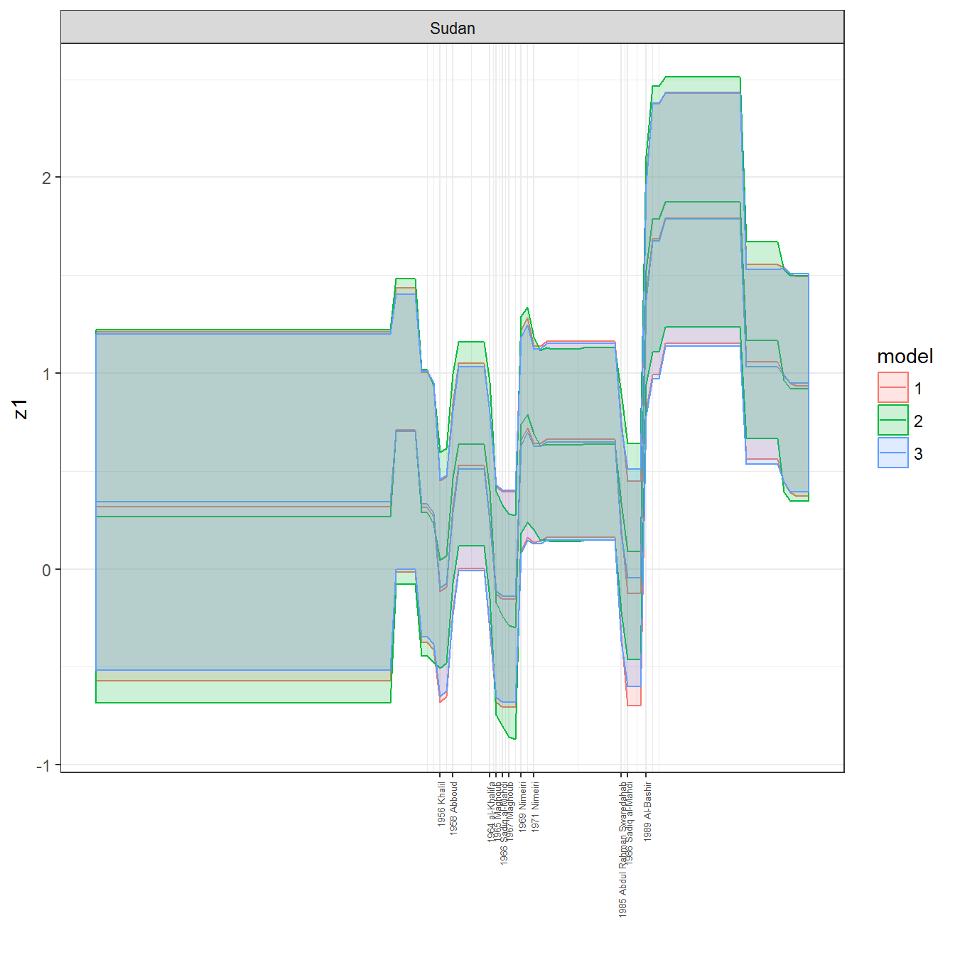
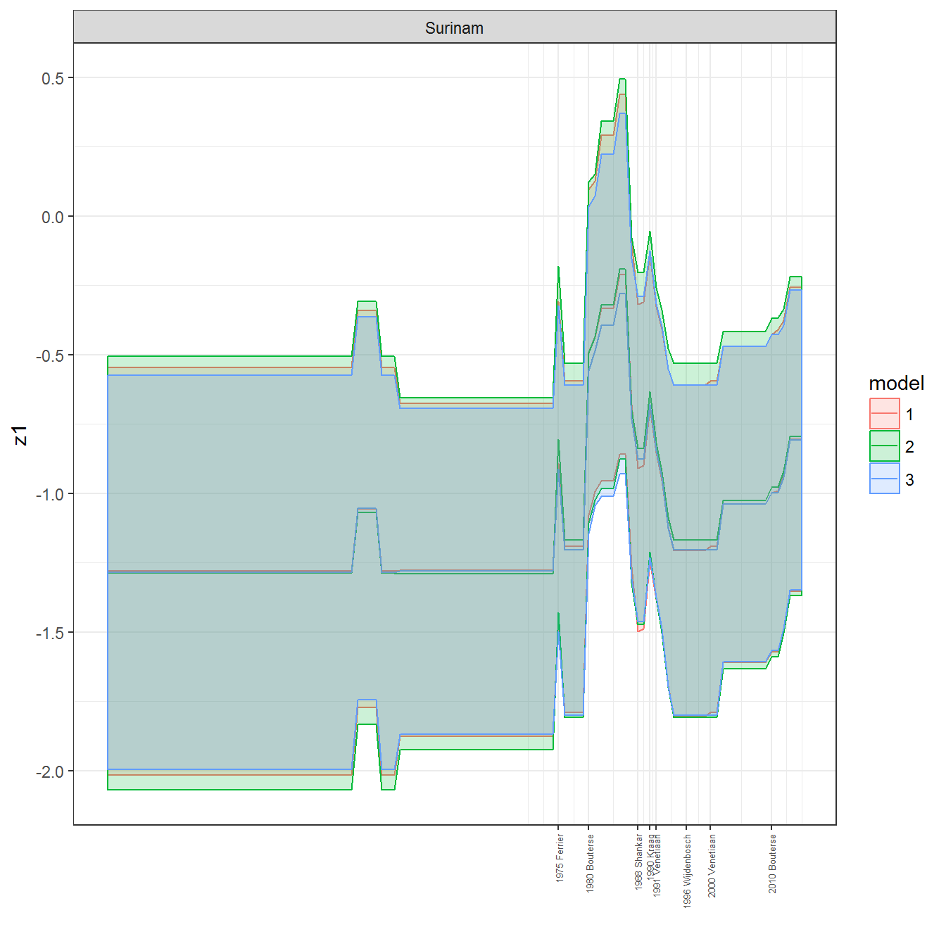
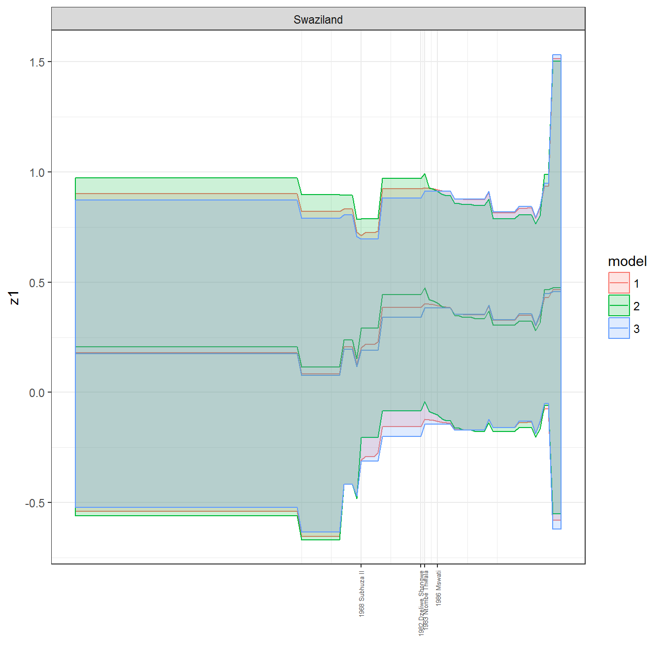
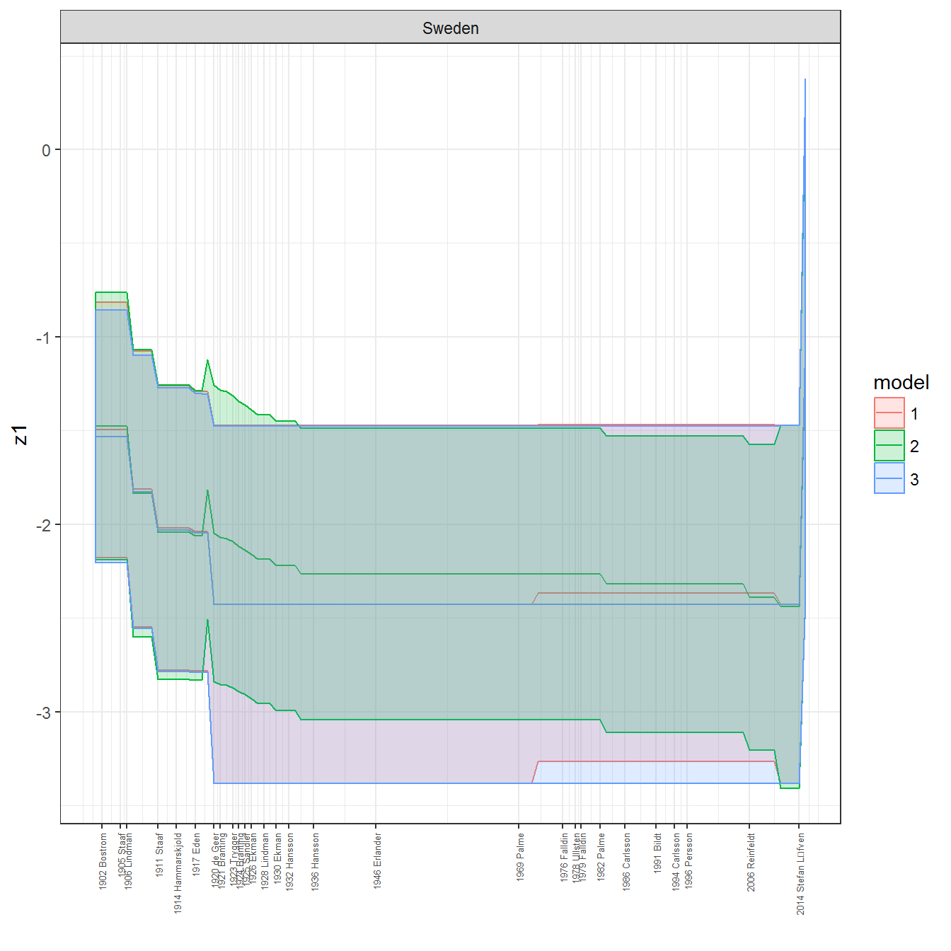
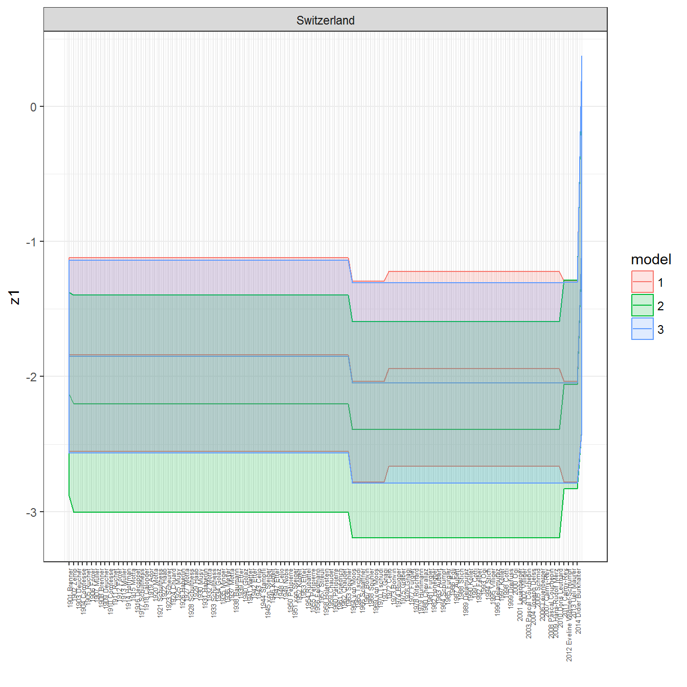
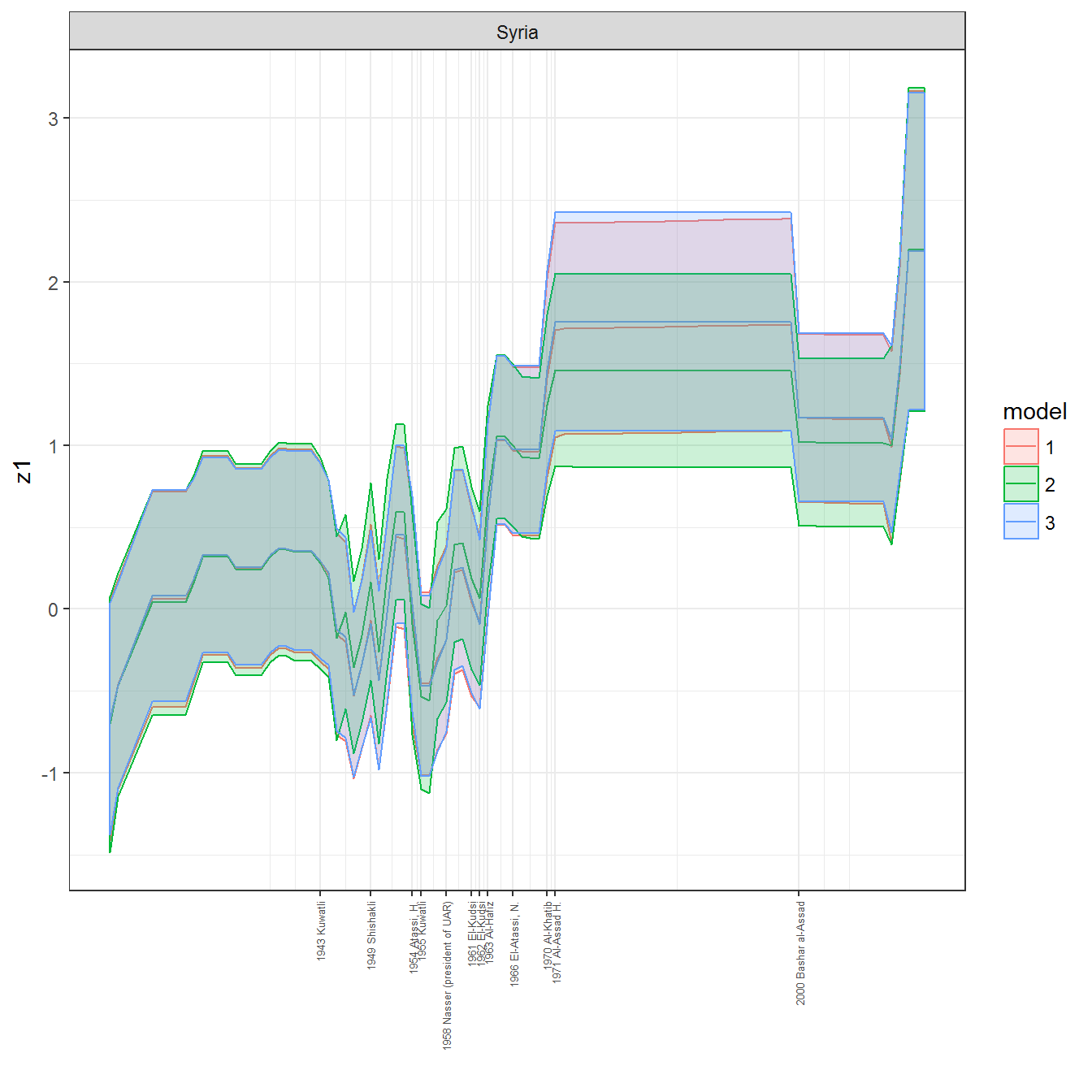
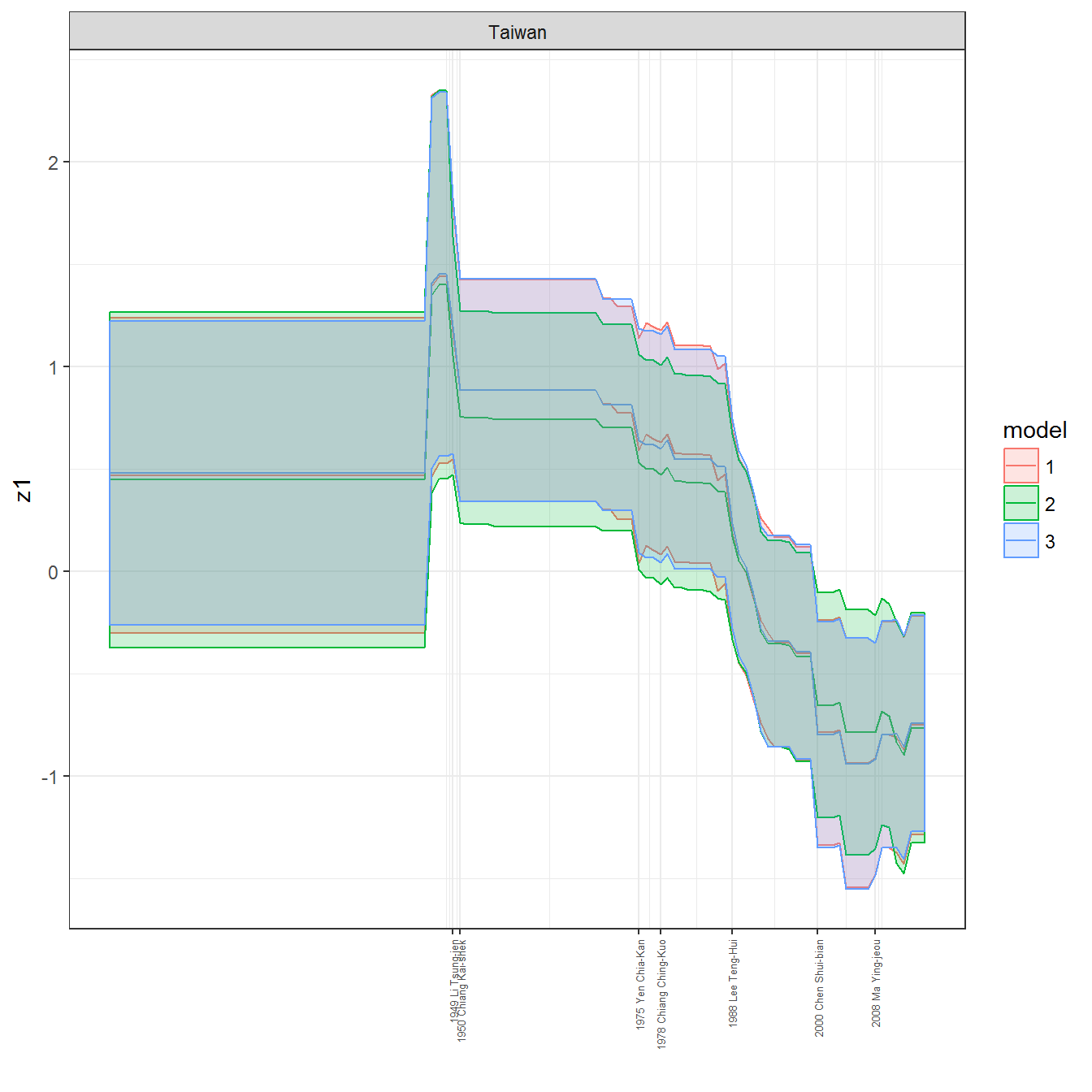
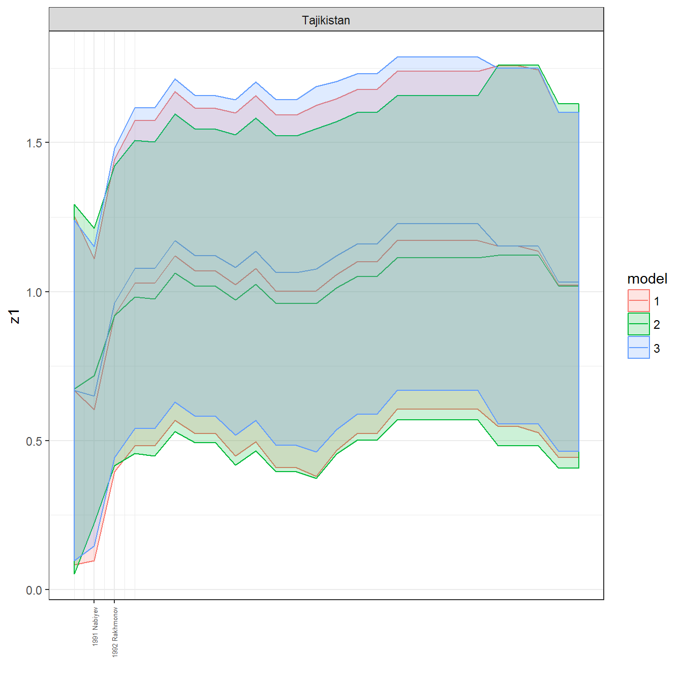
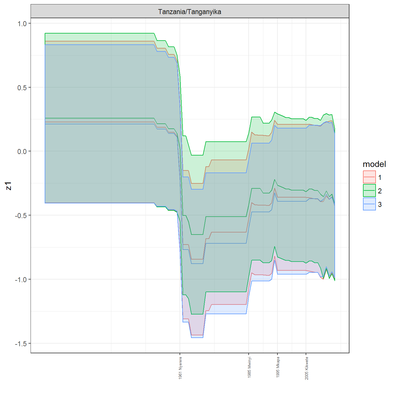
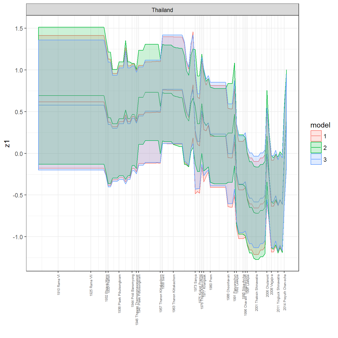
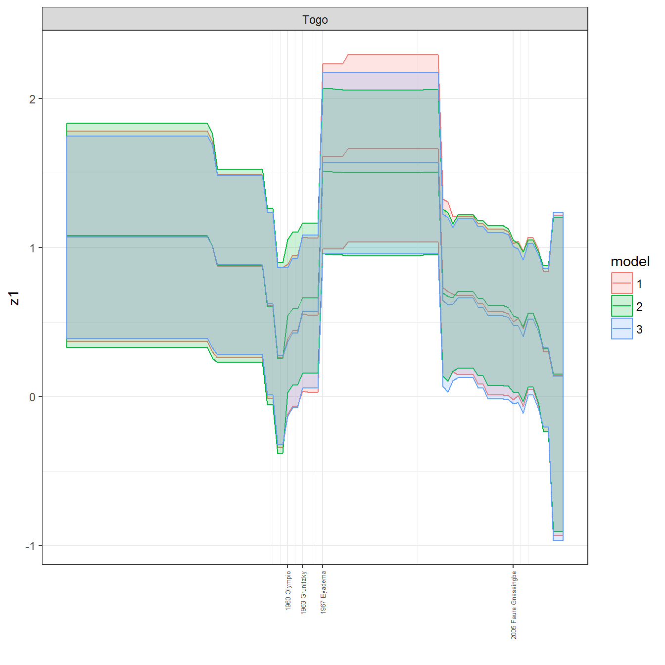
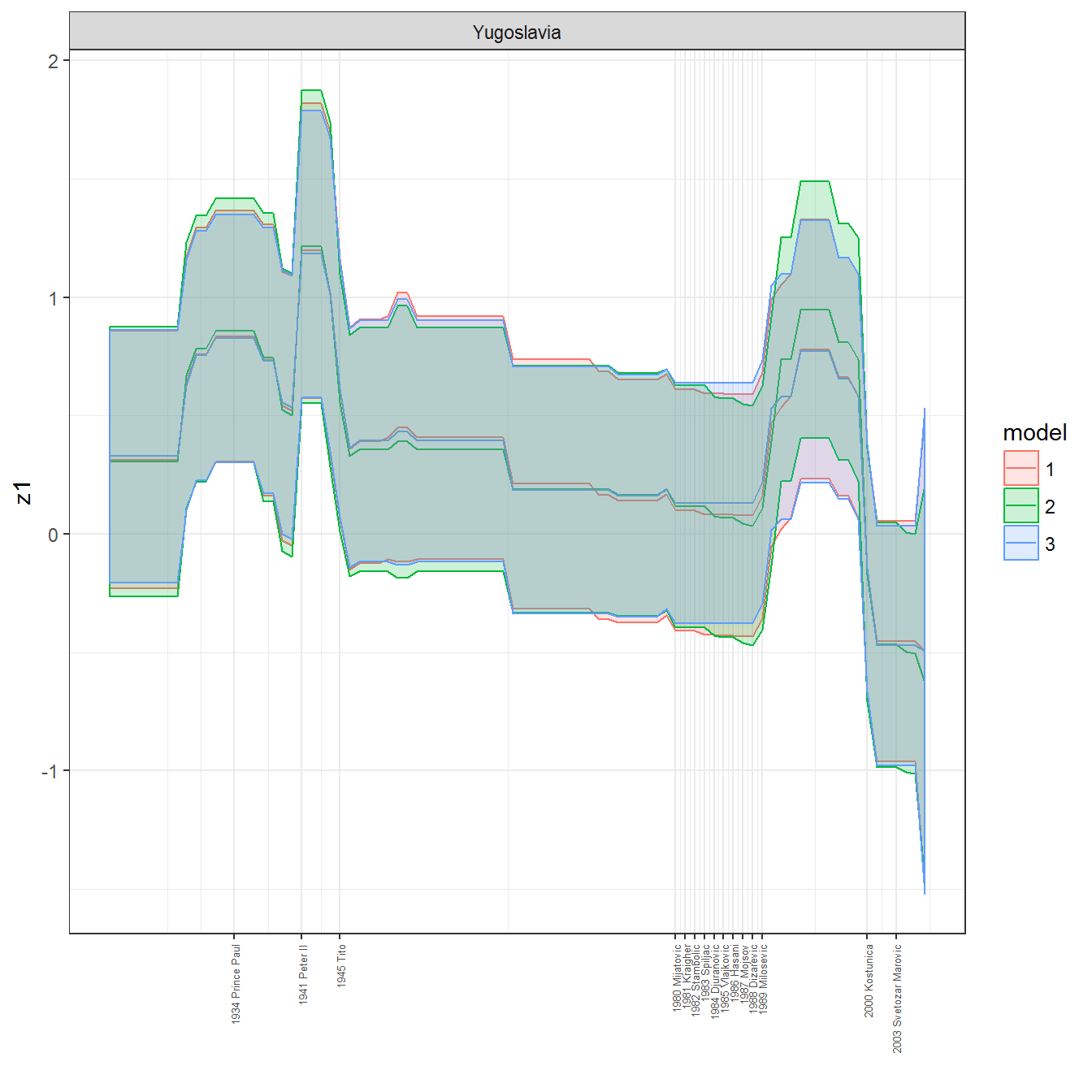
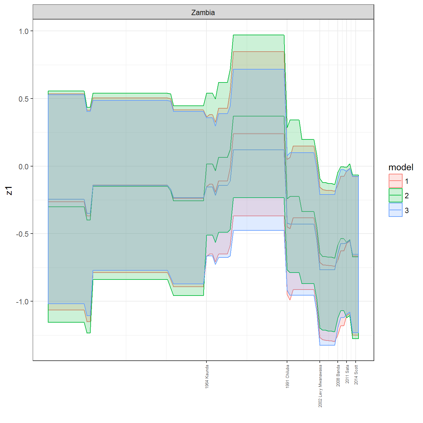
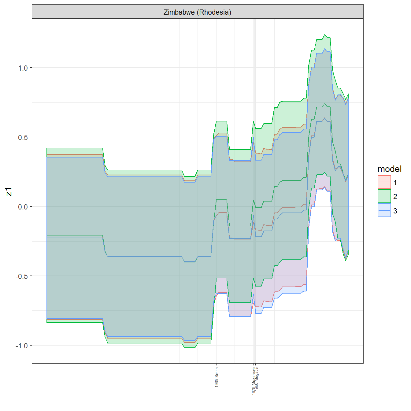
Full set of scores

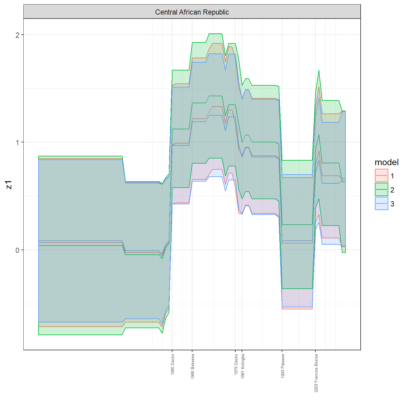
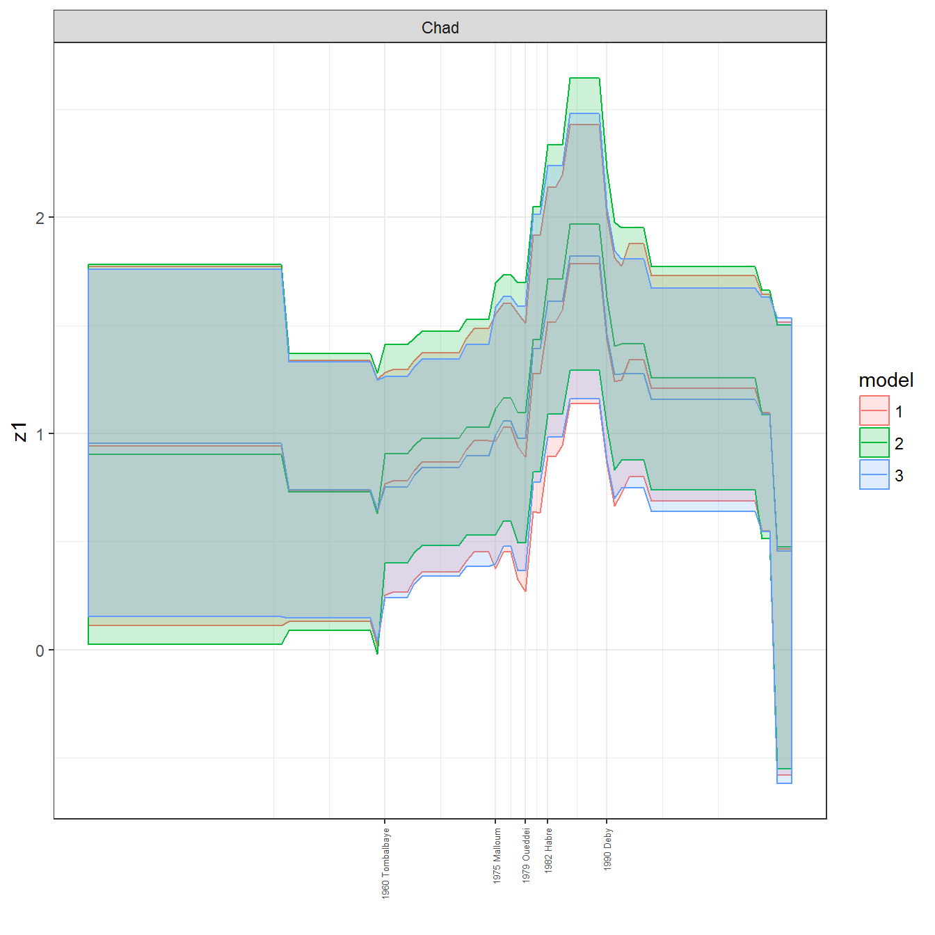
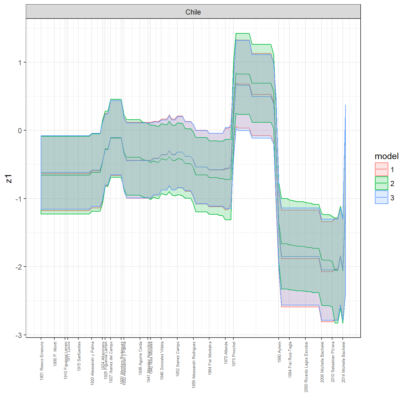
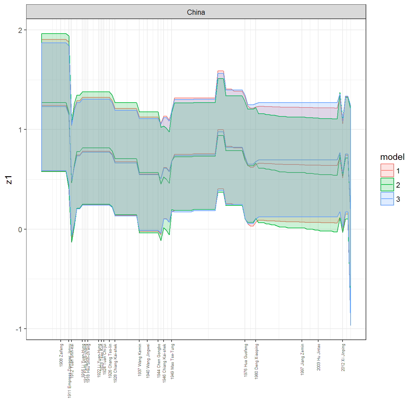
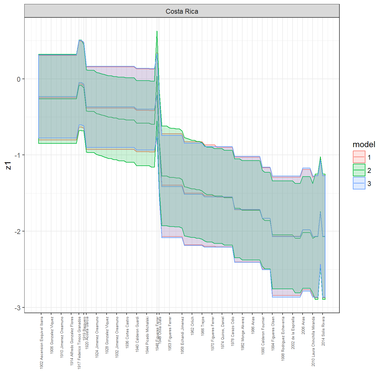
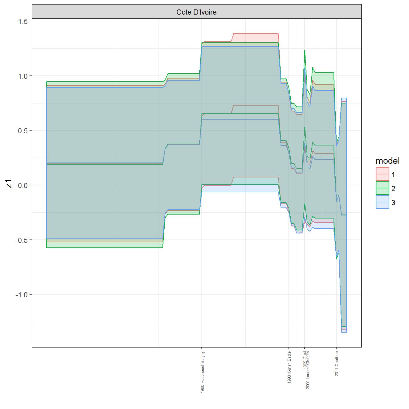
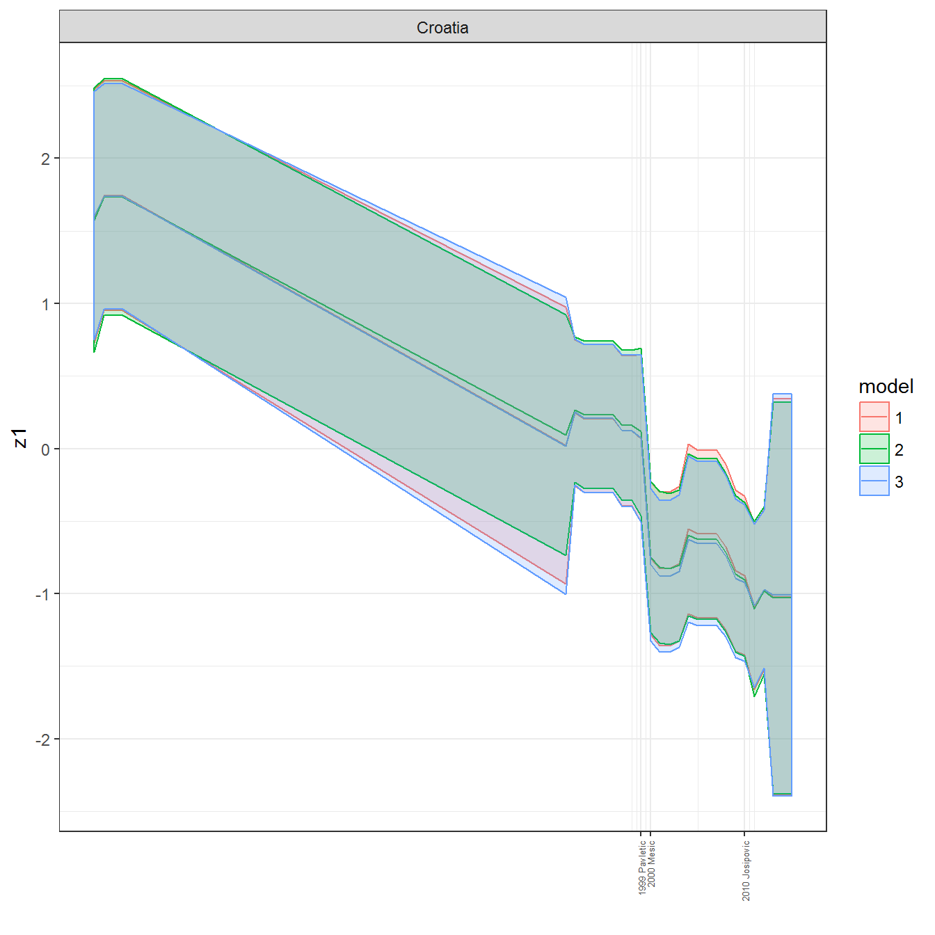
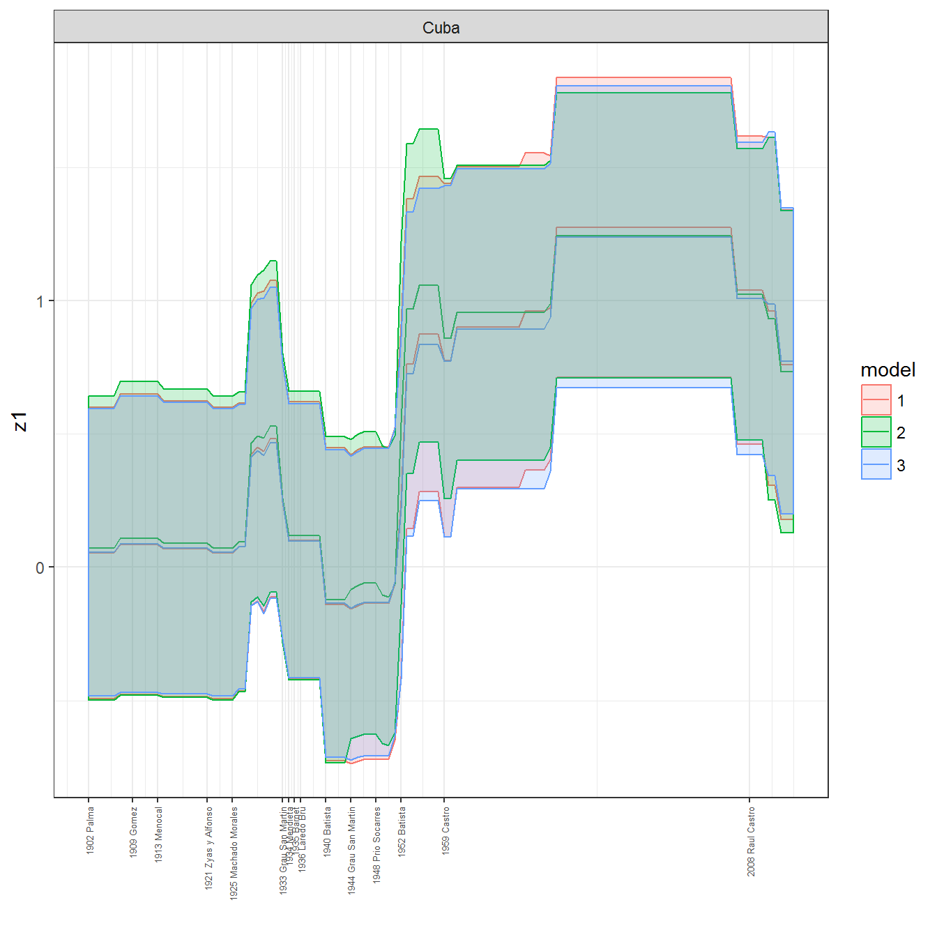
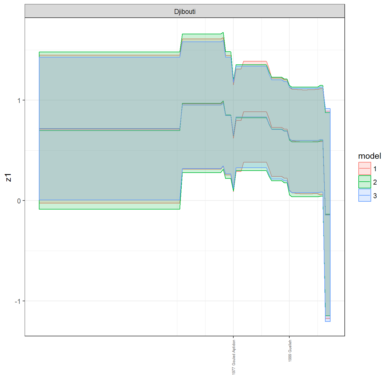
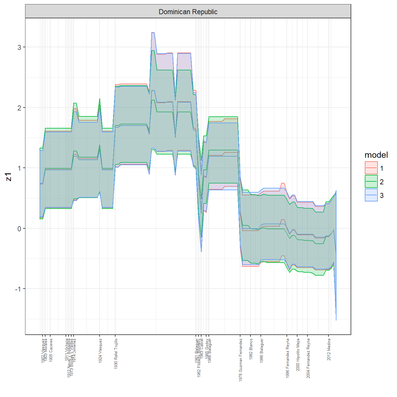
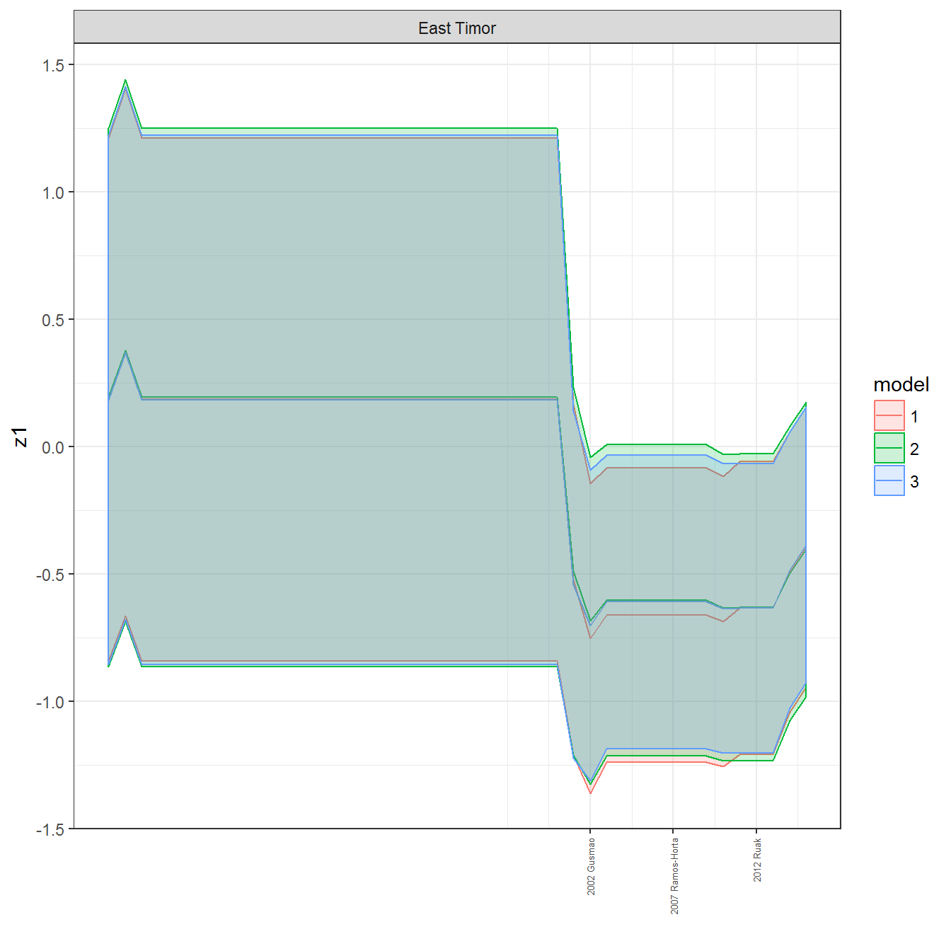
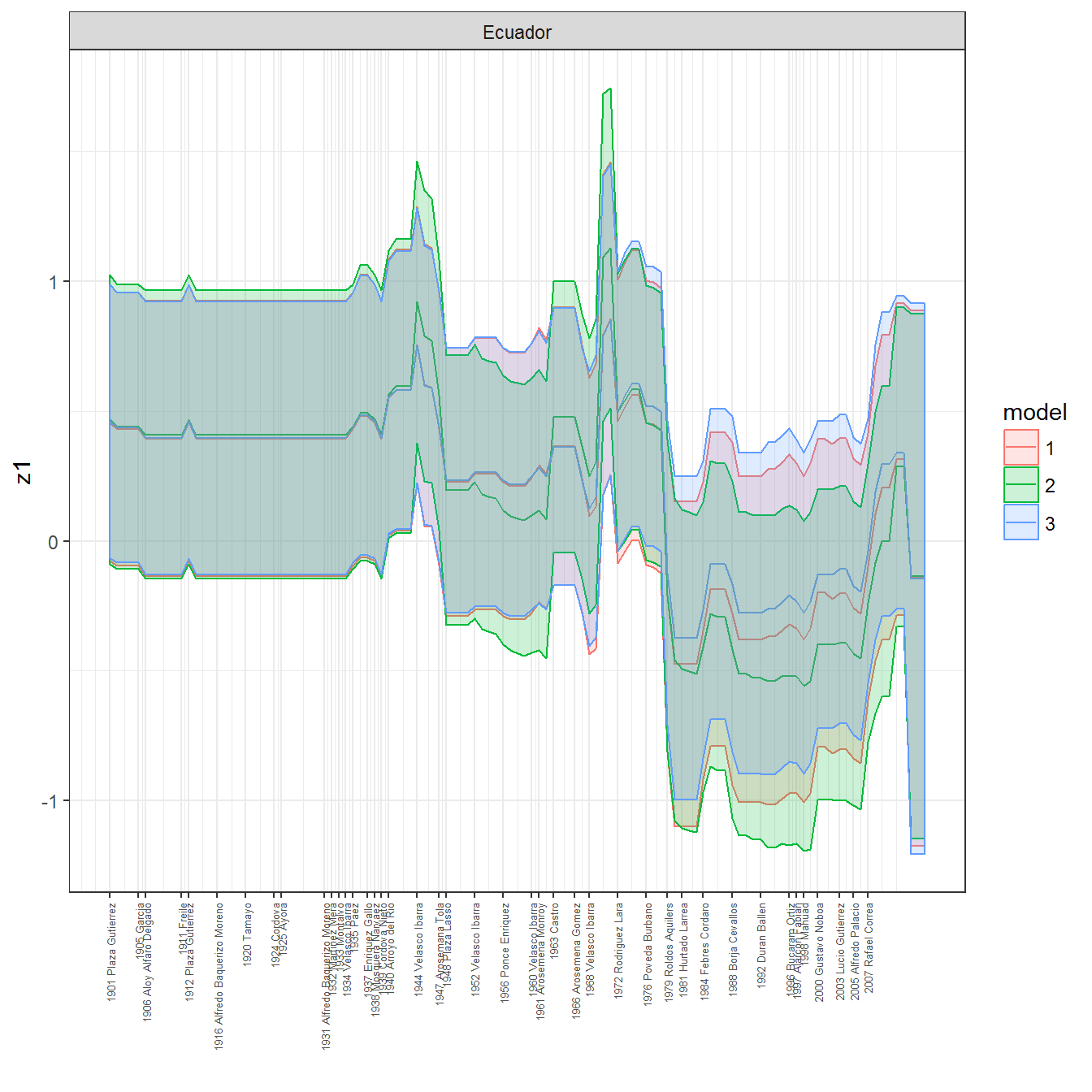
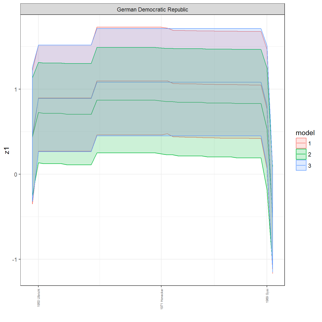
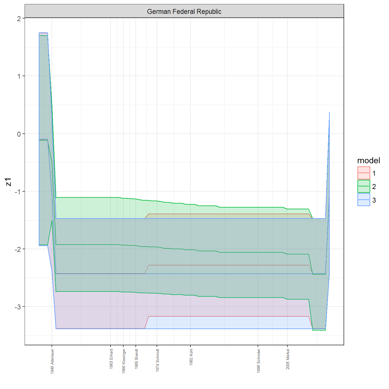
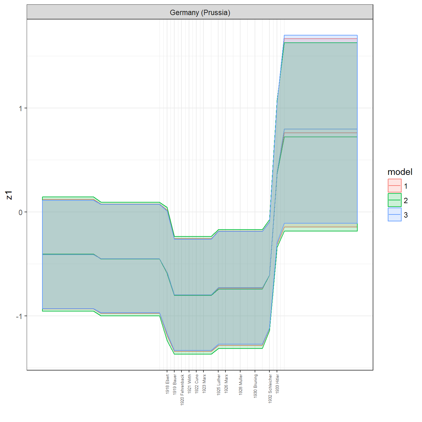
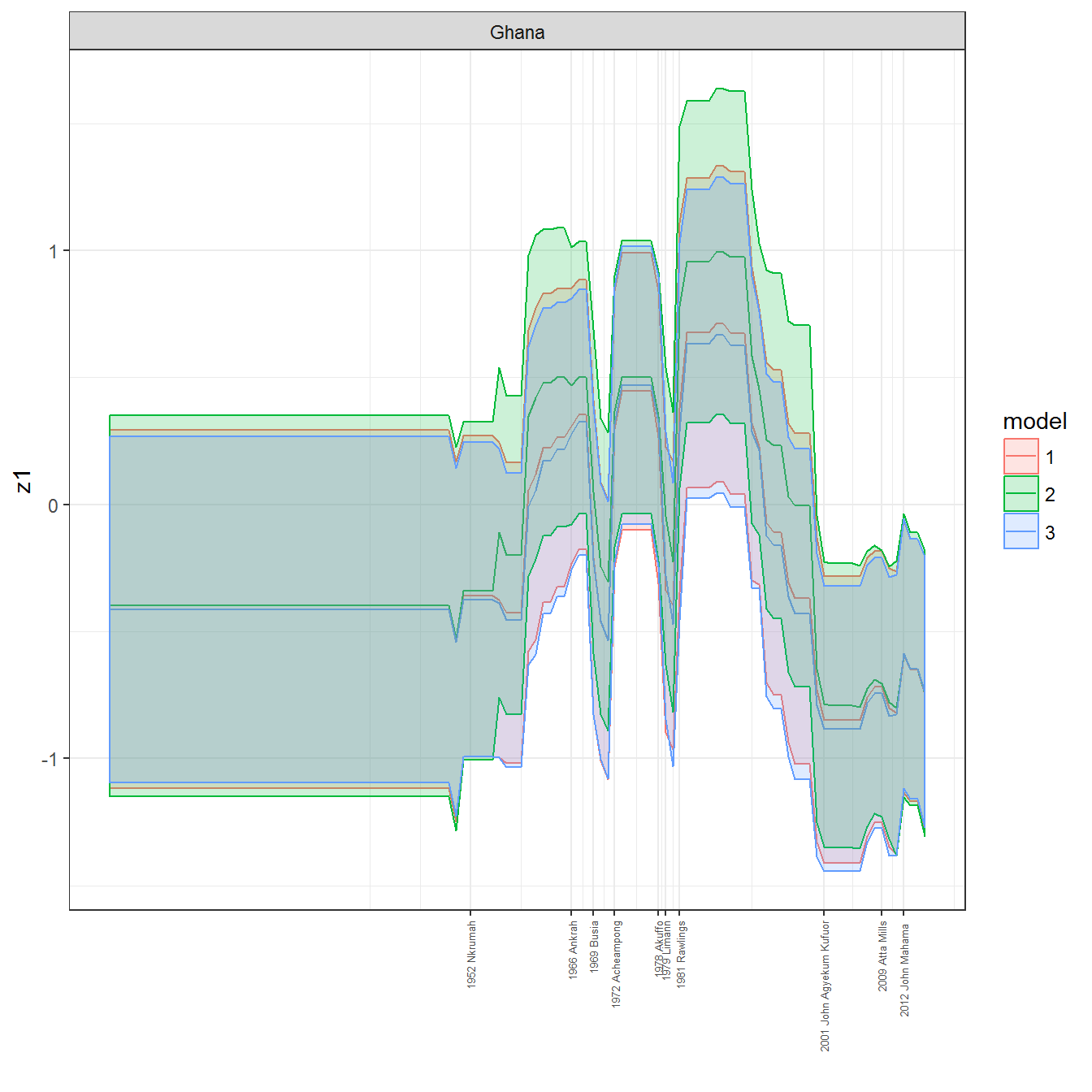
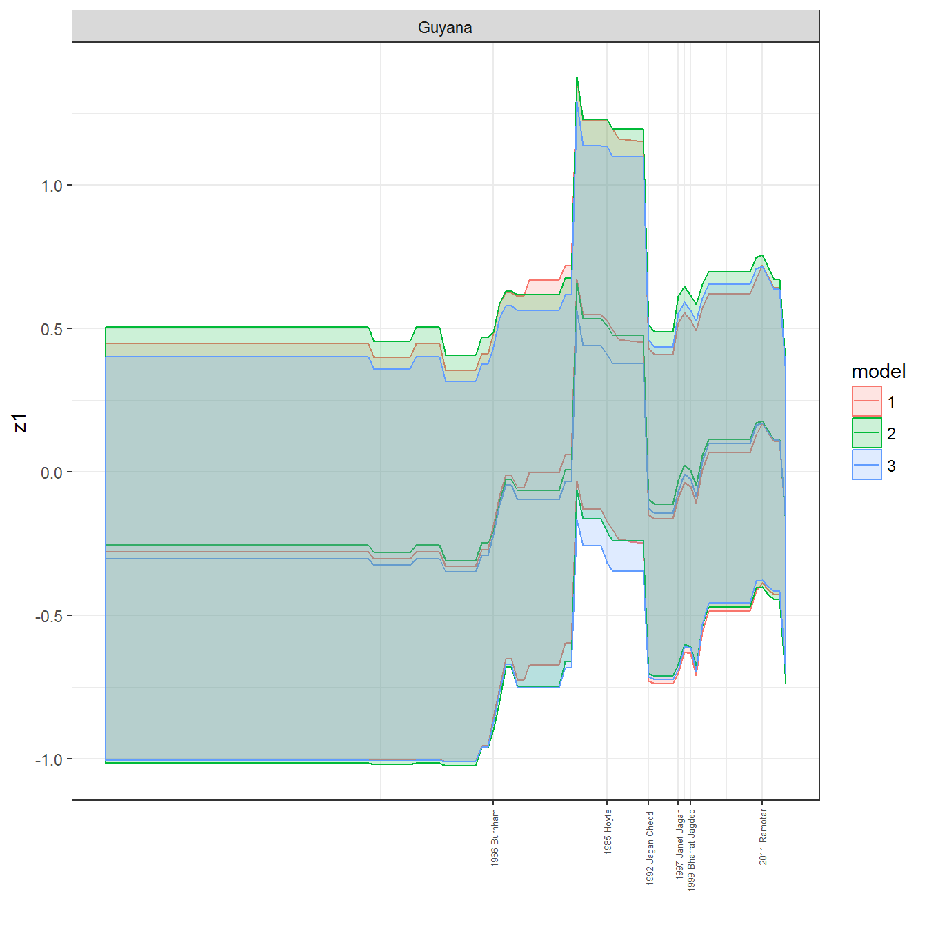
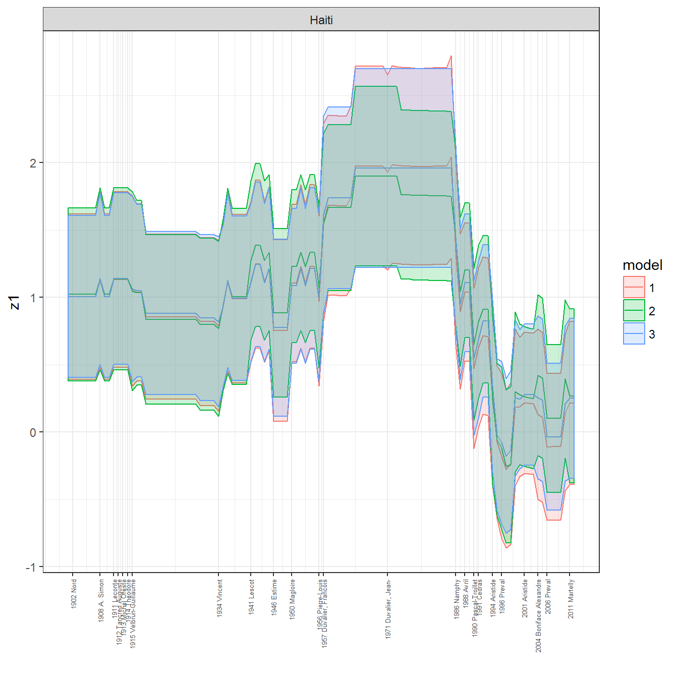
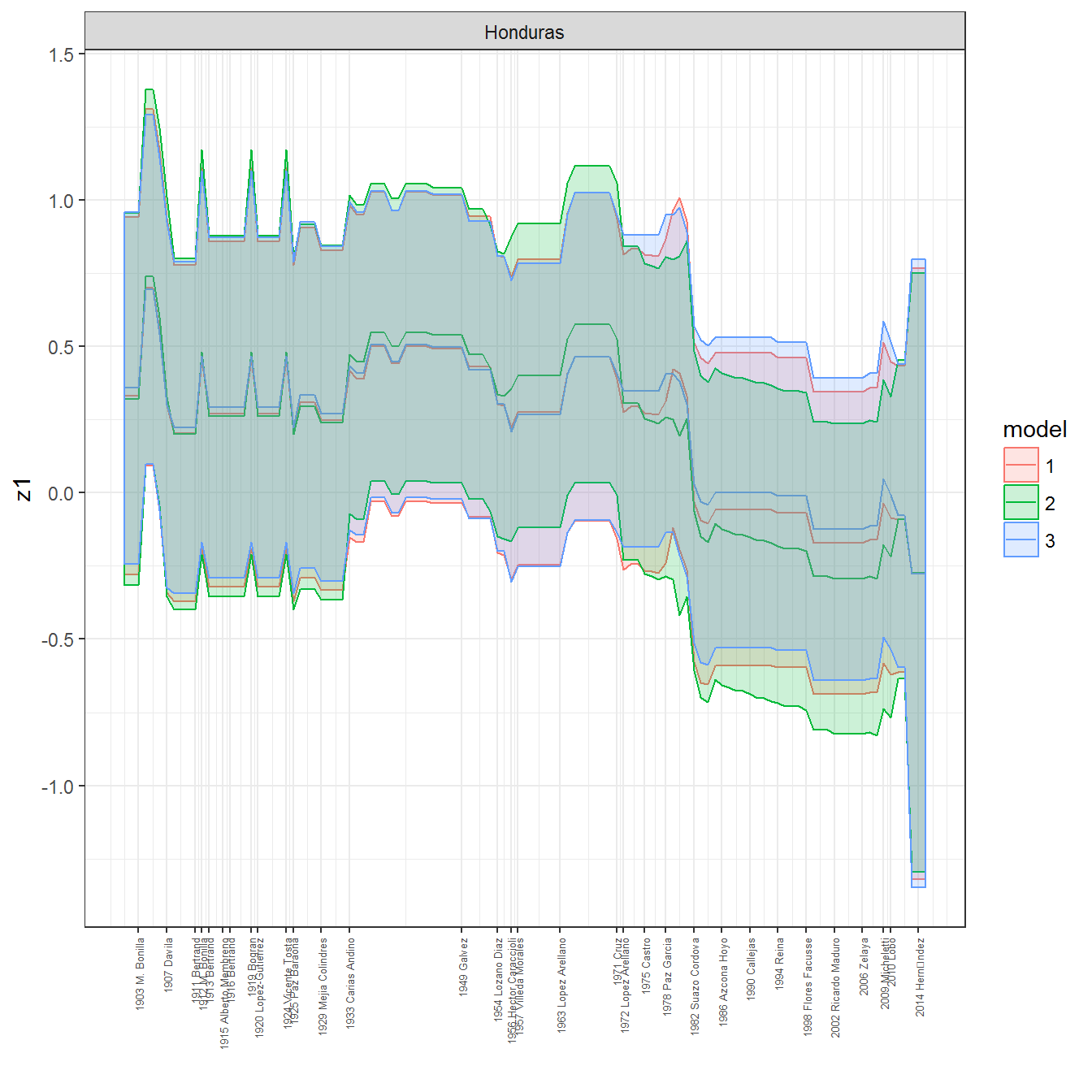
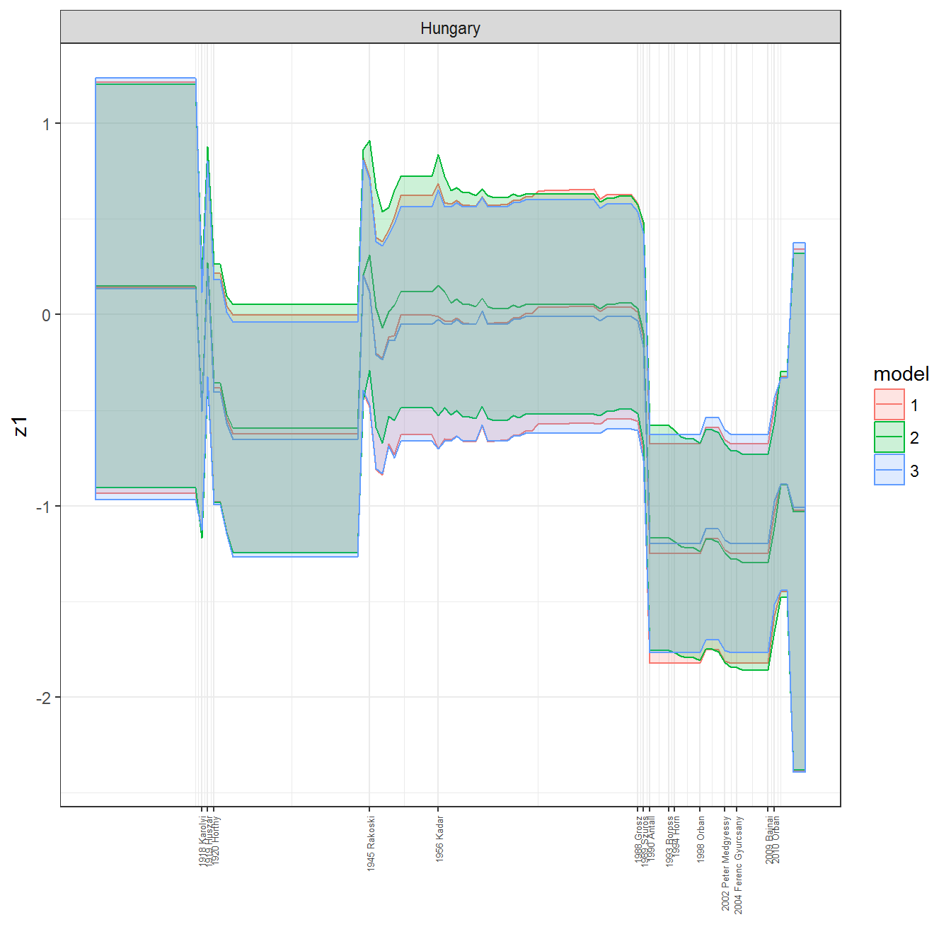
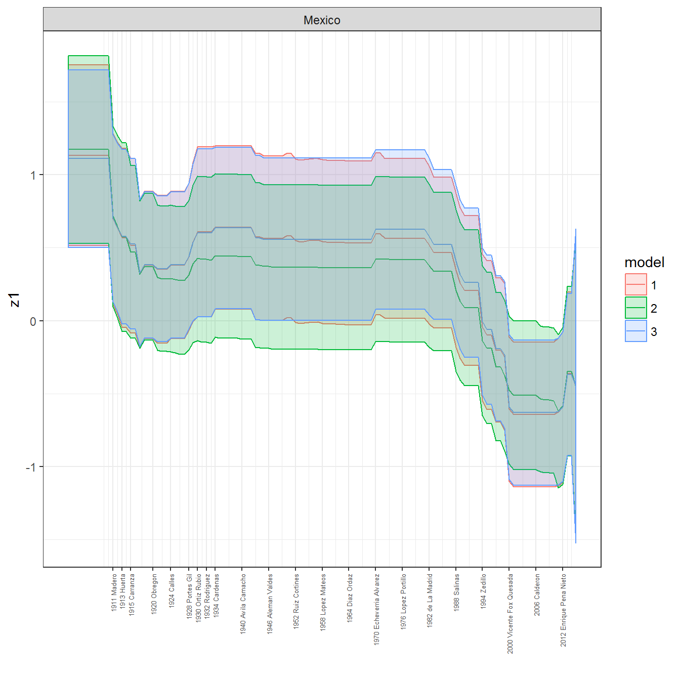
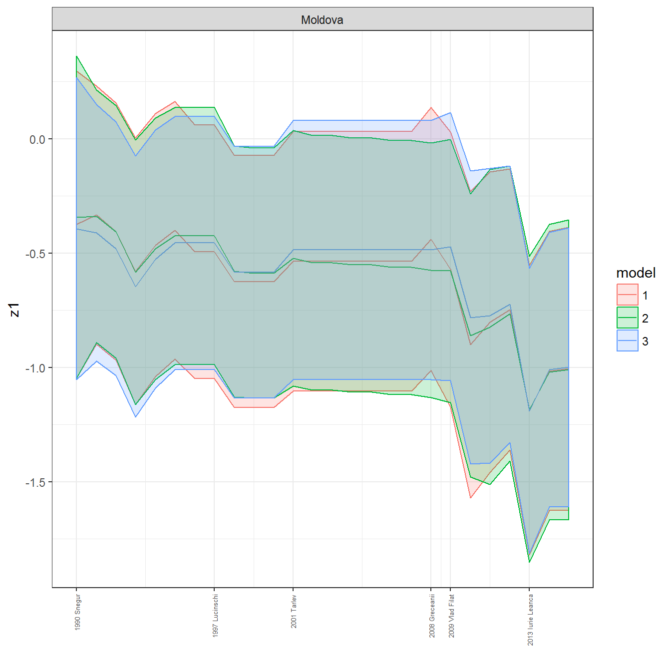
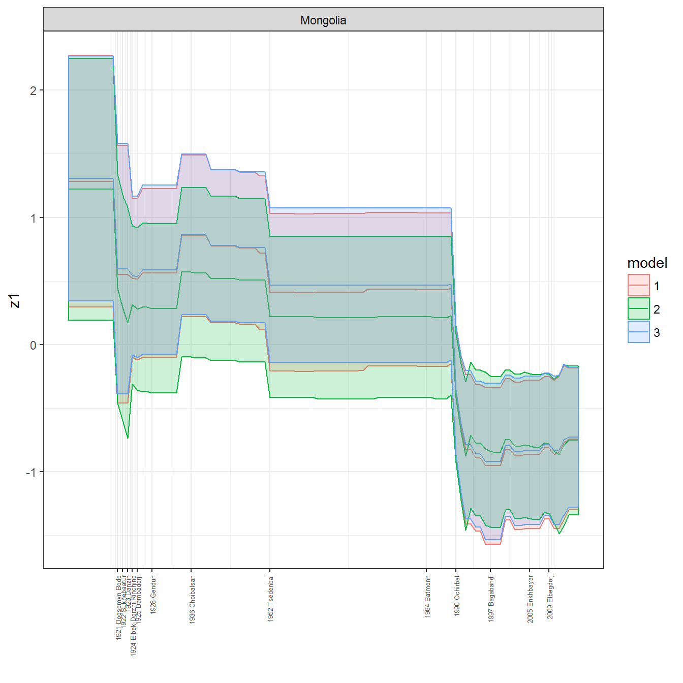
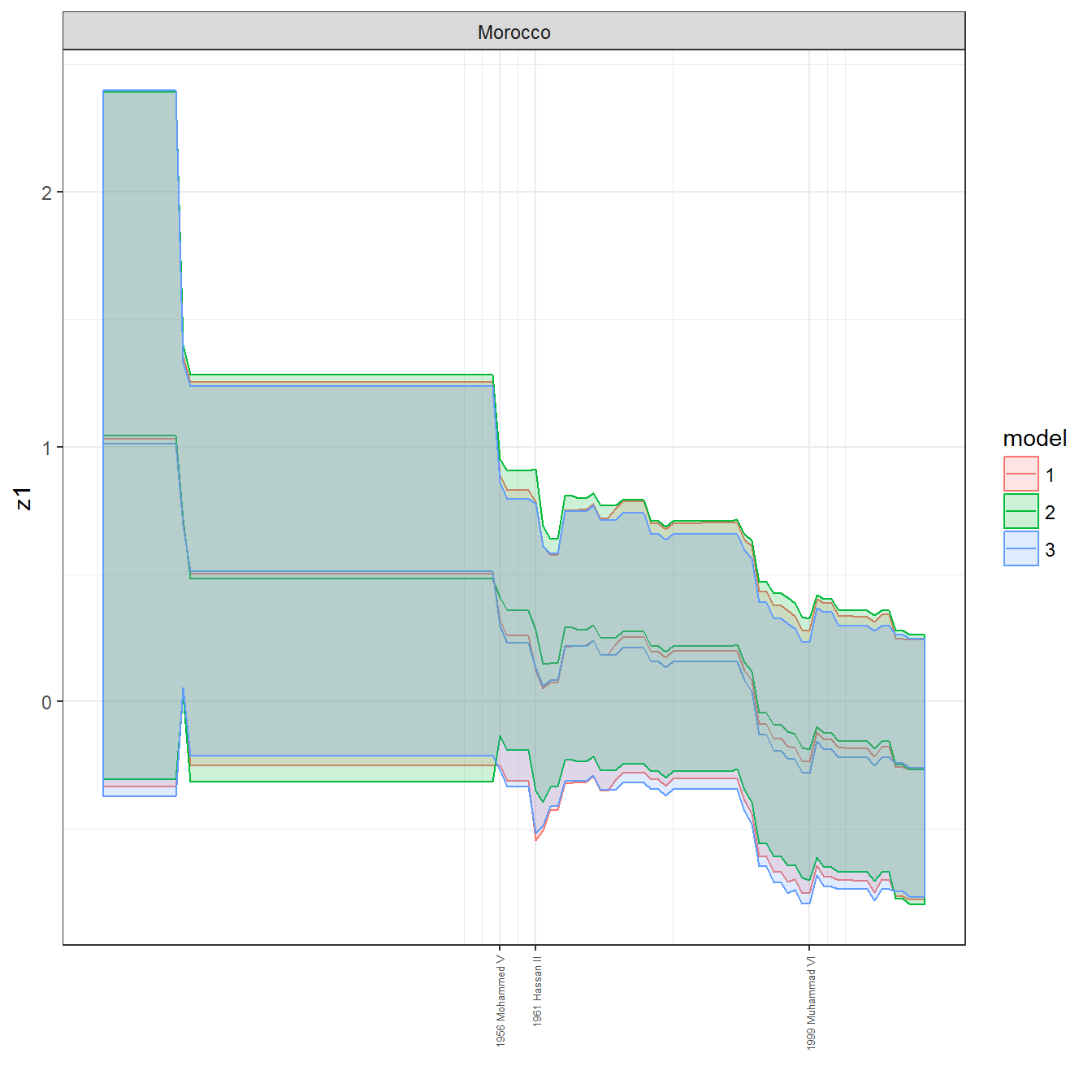
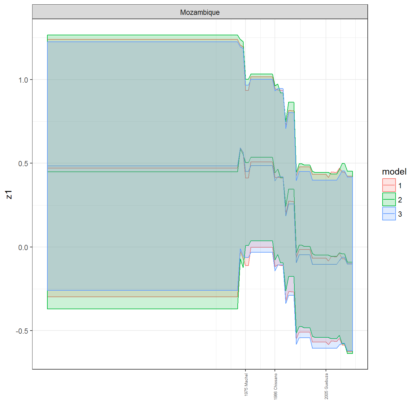
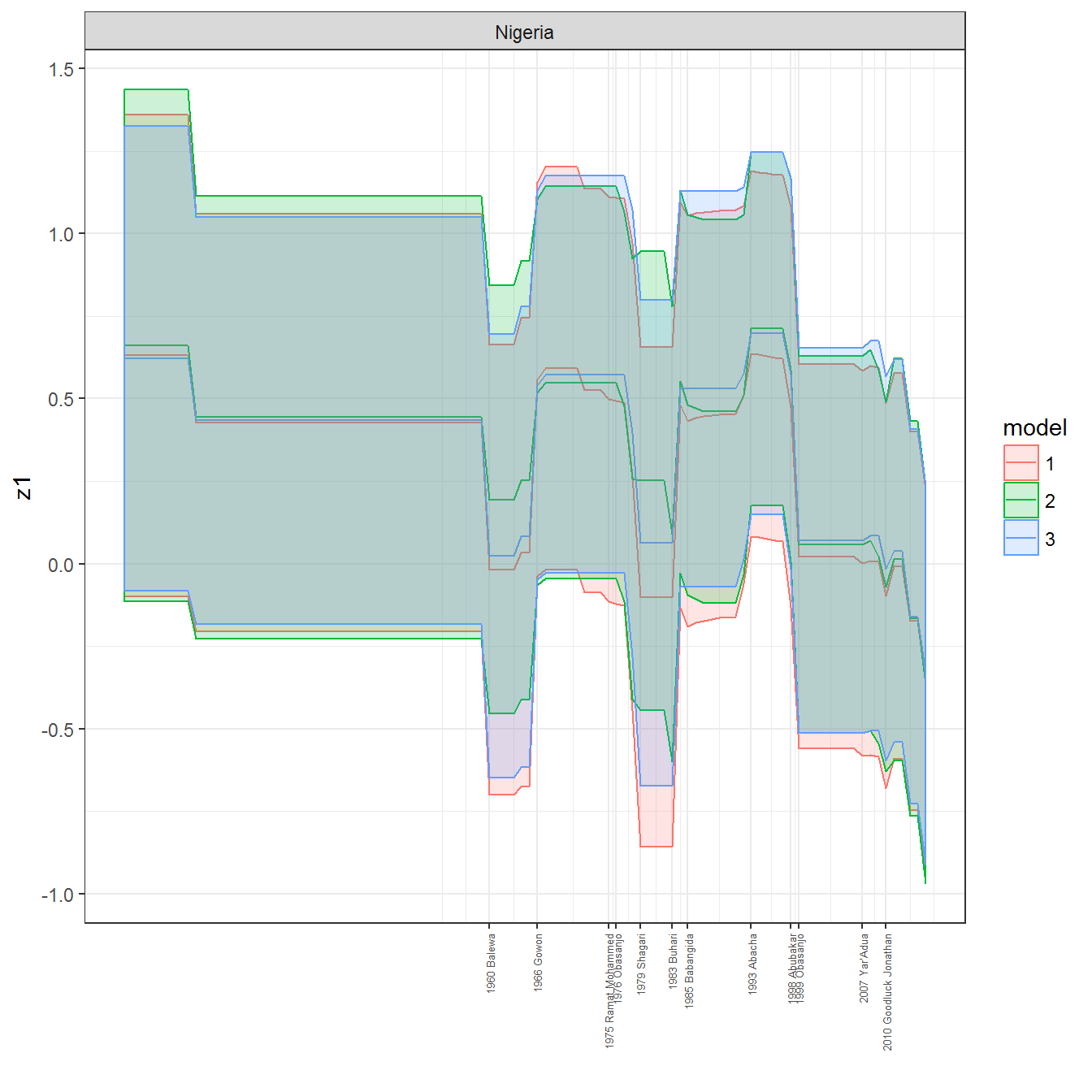
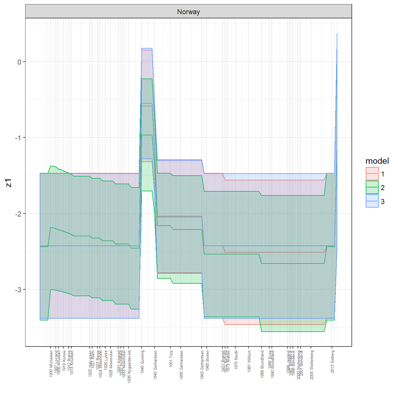
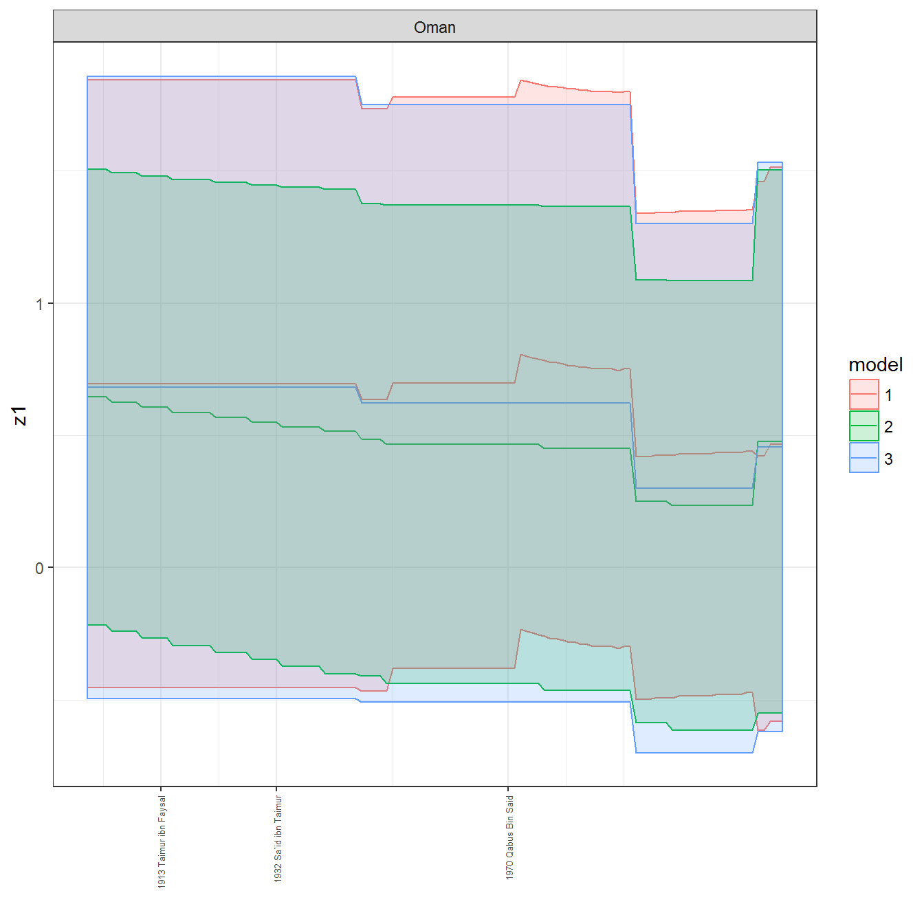
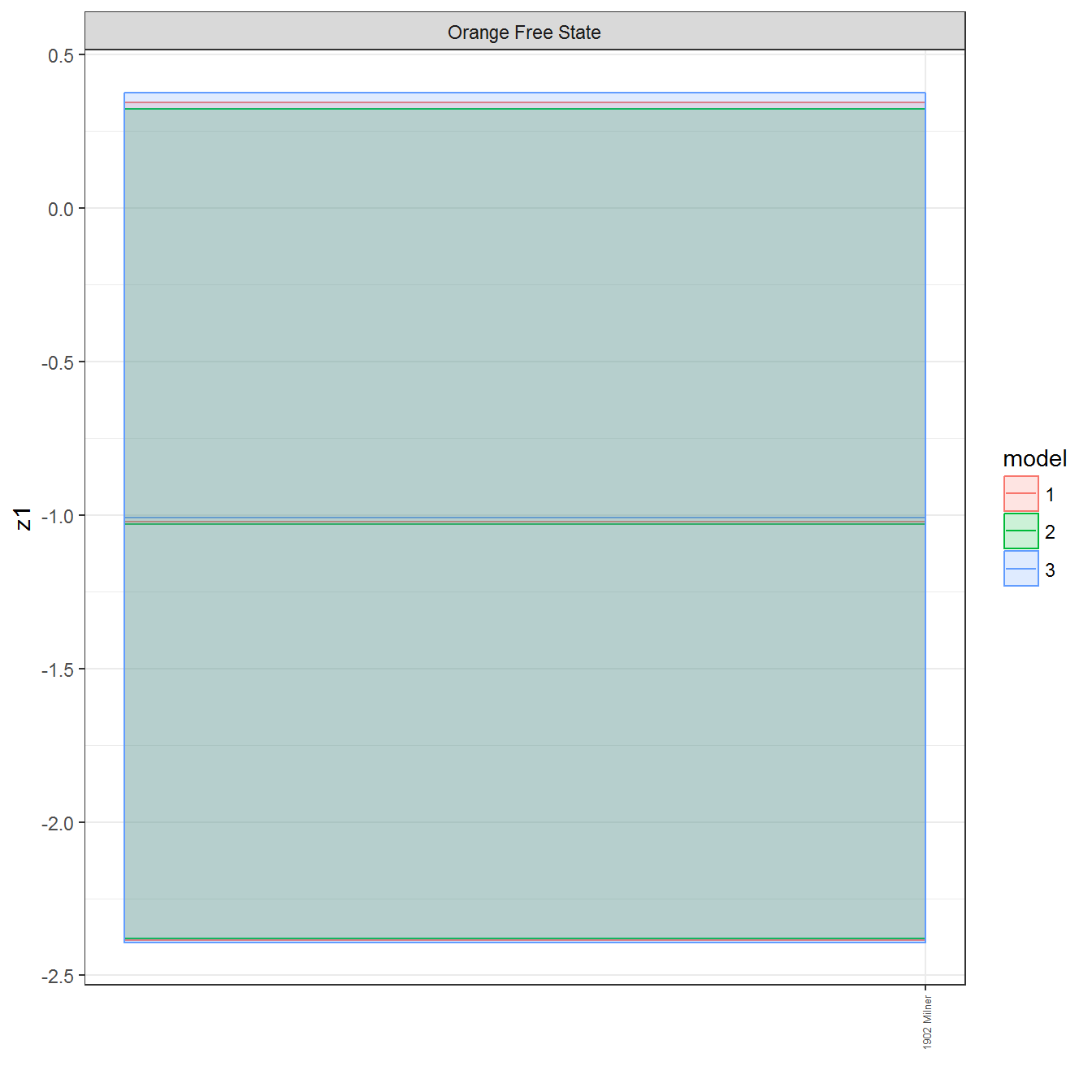
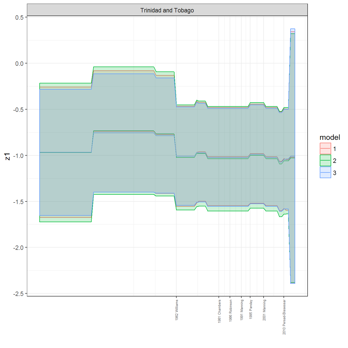
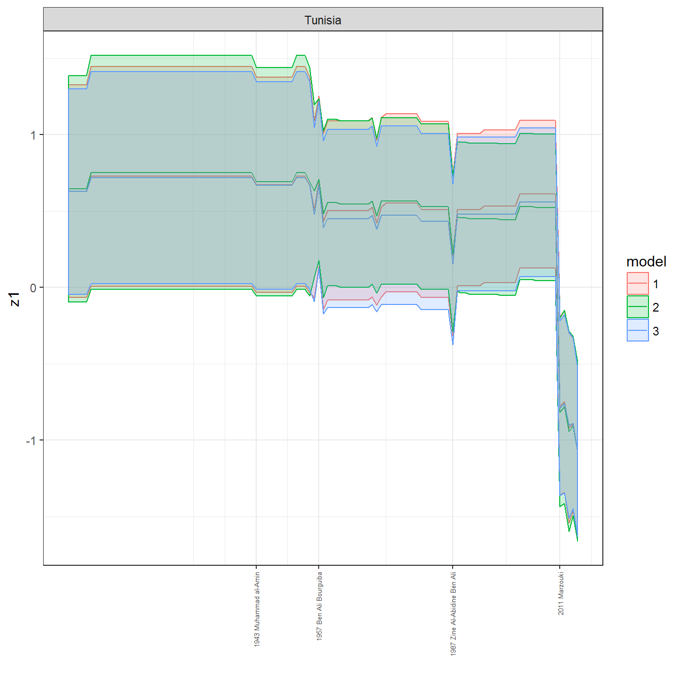
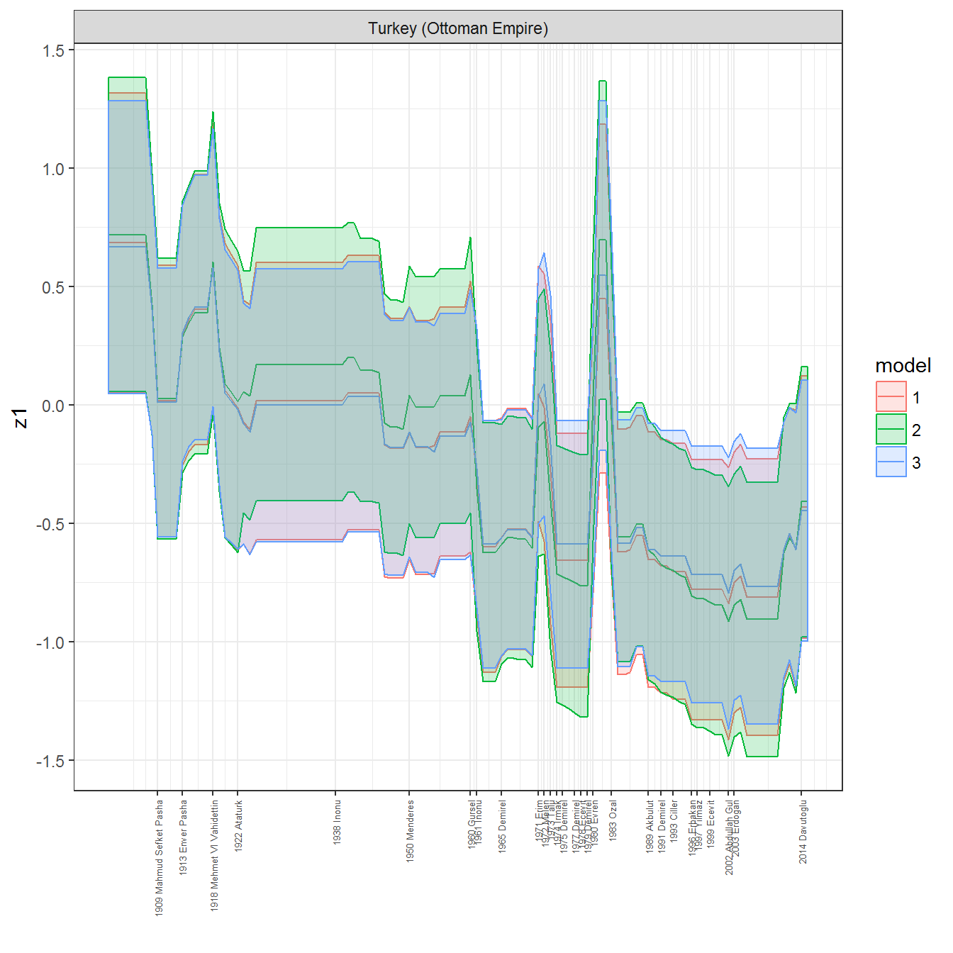
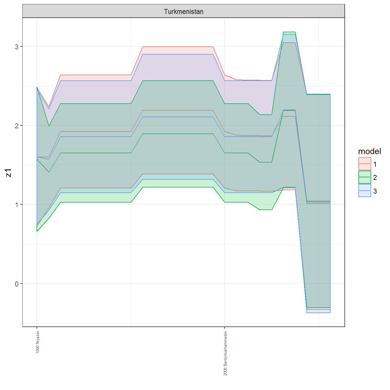
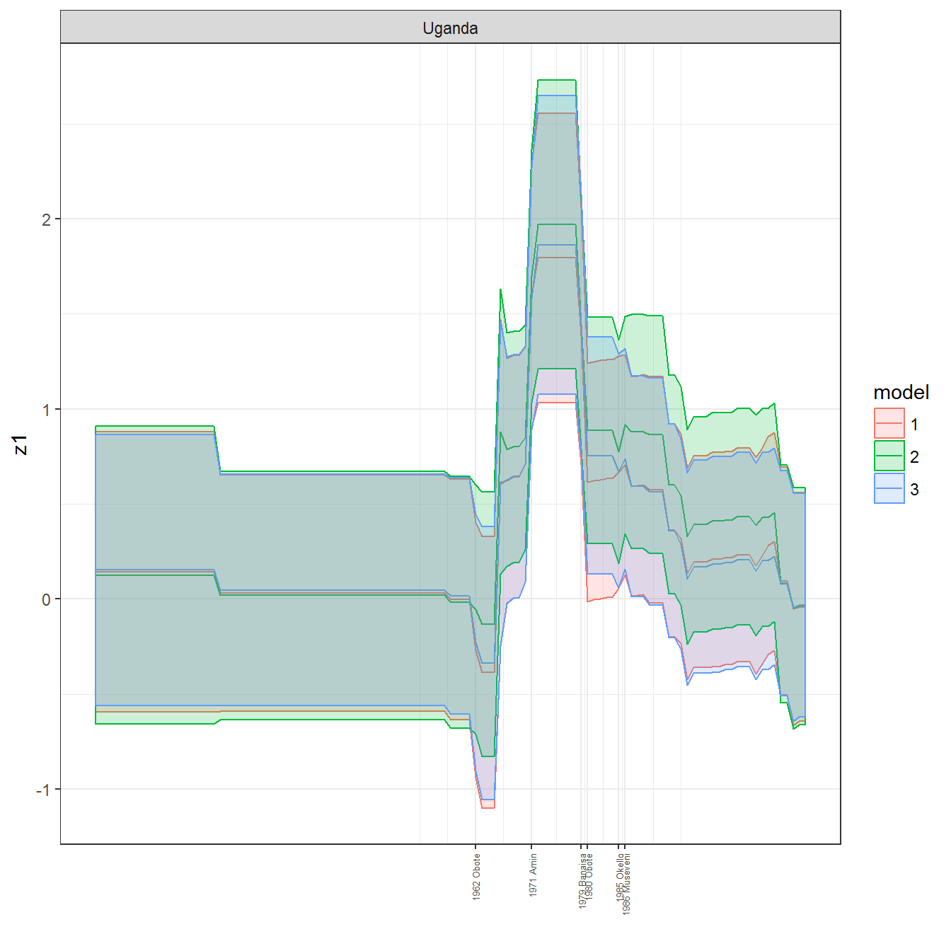
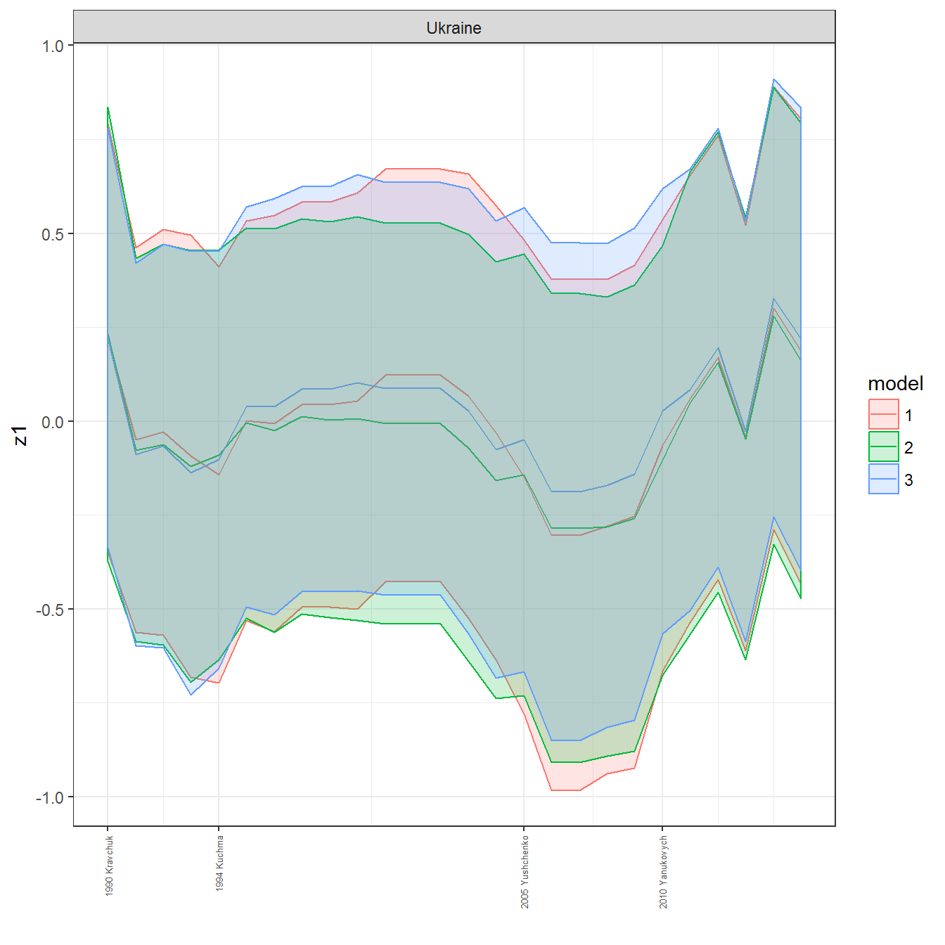
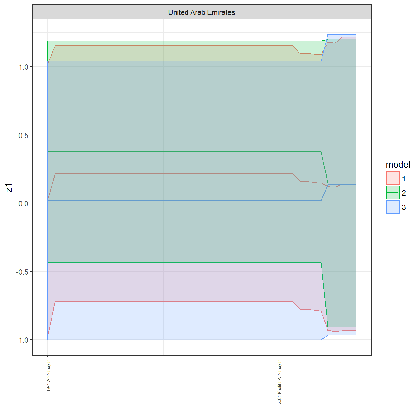
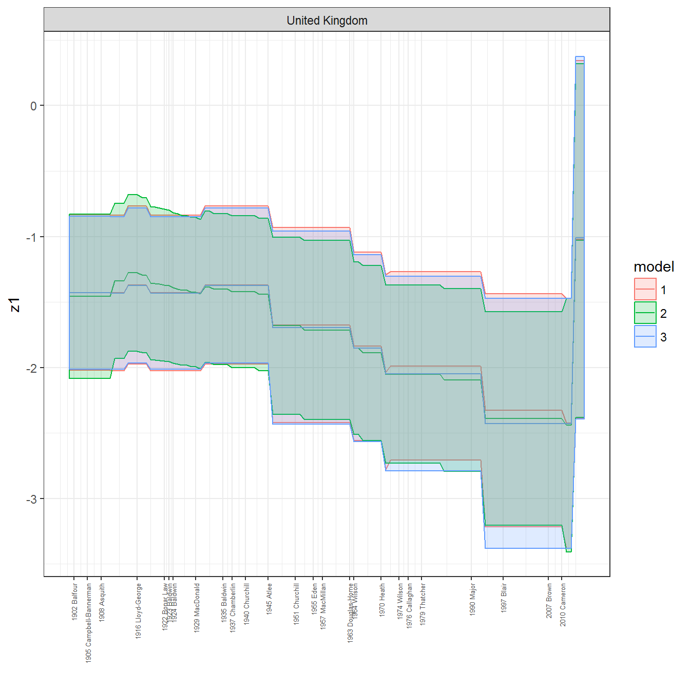
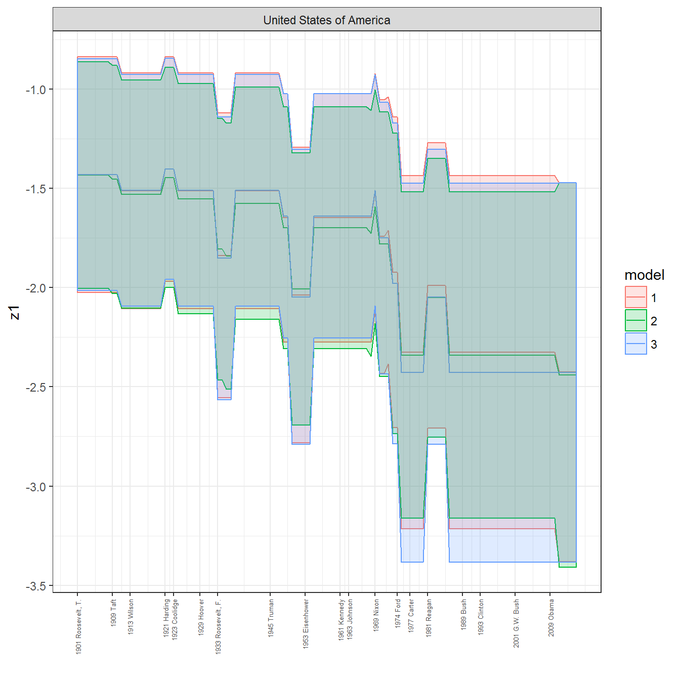
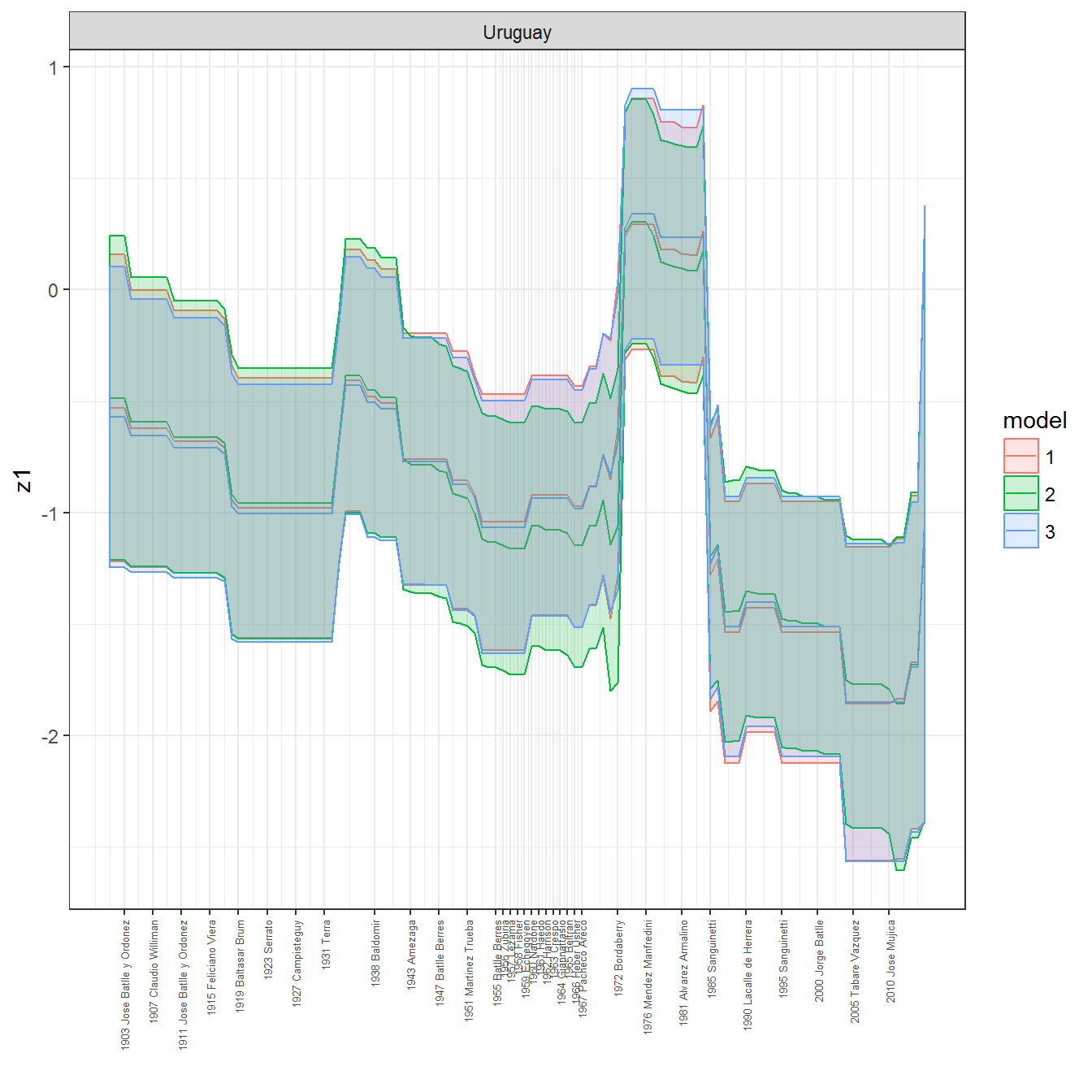
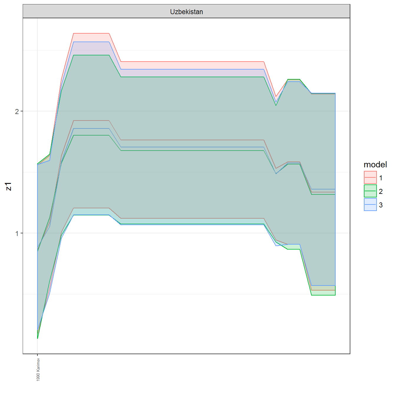
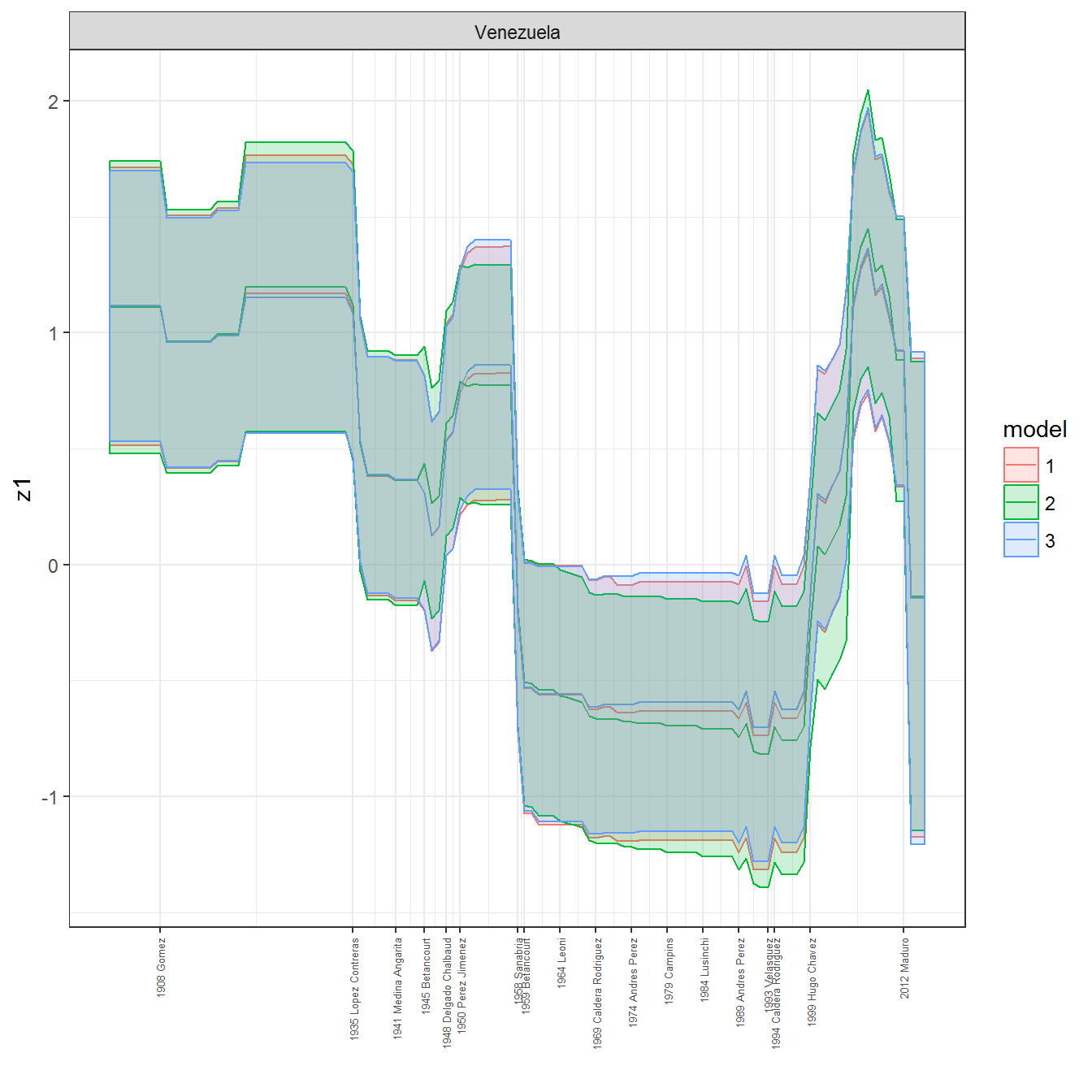
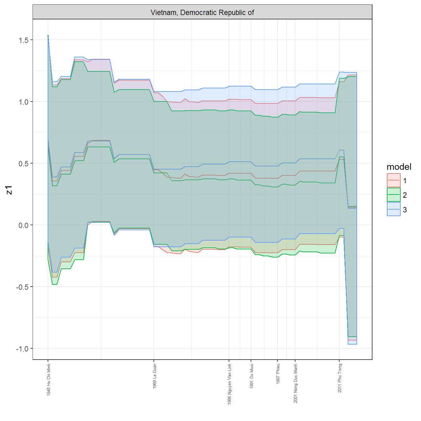
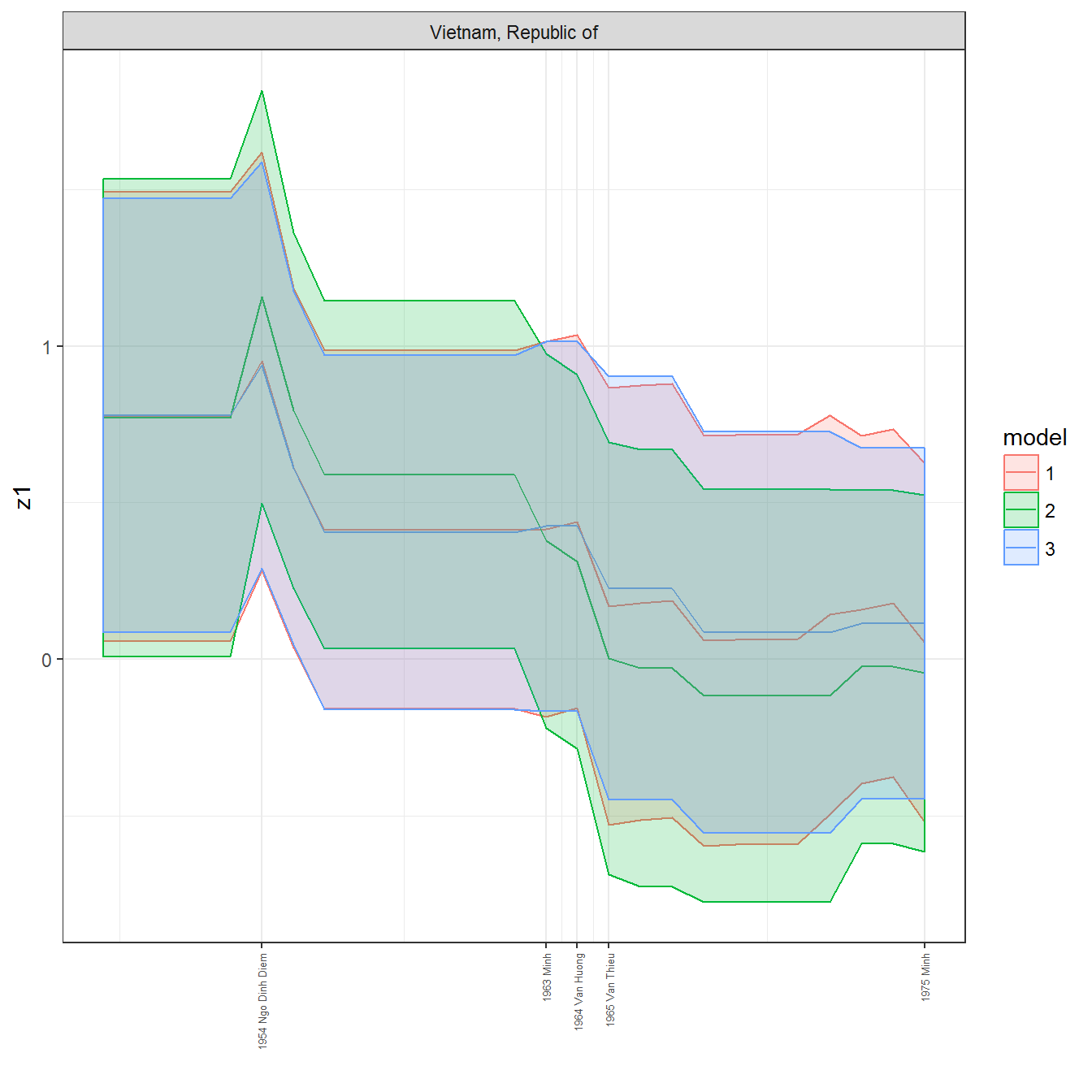
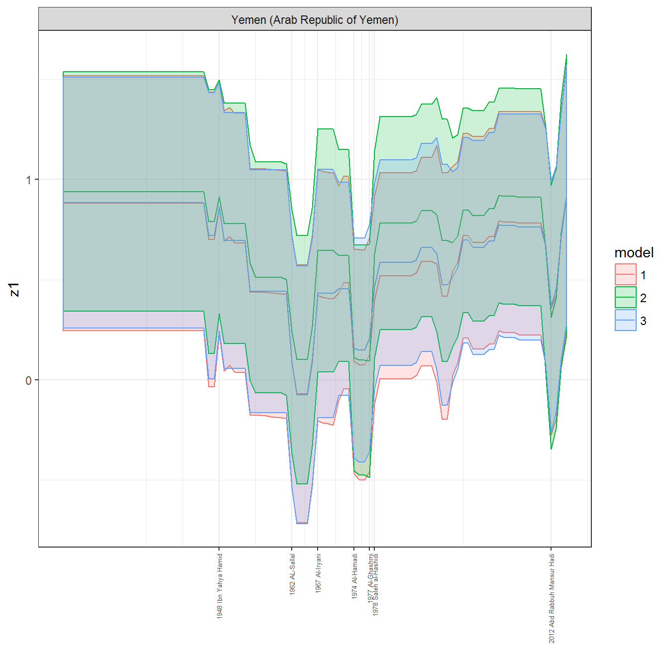
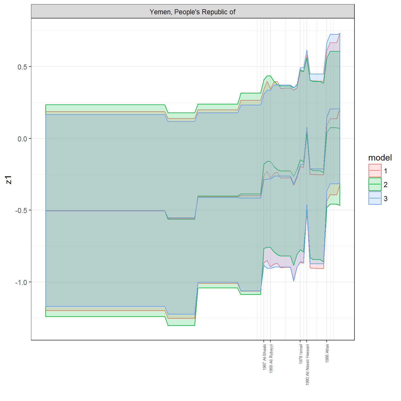
We can visualize the full set of scores (this takes a long time to run, so it is not run by default; set eval = TRUE to run the chunk when compiling the vignette):

library(lubridate)

# Visual test
leader_data <- archigos %>% 
  group_by(GWn, leader, startdate, enddate) %>%
  summarise(year = year(startdate)) %>%
  group_by(GWn, year) %>%
  filter(enddate == max(enddate), 
         startdate == max(startdate))


personal_data <- left_join(personal_scores,leader_data) %>%
  group_by(country_name, model) %>%
  arrange(model, country_name, year) %>%
  ungroup()

## Joining, by = c("GWn", "year")

for(country in unique(personal_data$country_name)) {

  data <- personal_data %>% filter(country_name %in% country, year > 1900)
  
  if(length(data$year[!is.na(data$leader)]) > 0) {
  p <- ggplot(data = data, aes(x=year,
                               y = z1, 
                               ymin = pct025, 
                               ymax = pct975,
                               color = model,
                               fill = model)) +
    geom_path() +
    geom_ribbon(alpha=0.2) +
    theme_bw() +
    scale_x_continuous(breaks = data$year[!is.na(data$leader) & data$model == 1 ],
                       labels = paste(data$year[!is.na(data$leader) & data$model == 1 ], 
                                      data$leader[!is.na(data$leader) & data$model == 1 ])) +
    theme(axis.text.x = element_text(angle = 90, 
                                     hjust = 1, 
                                     vjust = 0.5,
                                     size = 5)) +
    labs(x = "") +
    facet_wrap(~country_name, scales="free")
  
  print(p)
    
  }

}

References

Coppedge, Michael, John Gerring, Staffan I. Lindberg, Svend-Erik Skaaning, Jan Teorell, David Altman, Michael Bernhard, et al. 2016. “V-Dem [Country-Year/Country-Date] Dataset, Version 6.1.” Dataset. Varieties of Democracy (V-Dem) Project. https://www.v-dem.net/en/data/data-version-6-1/.

Geddes, Barbara, Joseph Wright, and Erica Frantz. 2014. “Autocratic Breakdown and Regime Transitions: A New Data Set.” Perspectives on Politics 12 (1): 313–31. doi:10.1017/S1537592714000851.

Goemans, Henk, Kristian Gleditsch, and Giacomo Chiozza. 2009. “Introducing Archigos: A Dataset of Political Leaders.” Journal of Peace Research 46 (2): 269–83.

Kailitz, Steffen. 2013. “Classifying Political Regimes Revisited: Legitimation and Durability.” Democratization 20 (1): 39–60. doi:10.1080/13510347.2013.738861.

Magaloni, Beatriz, Jonathan Chu, and Eric Min. 2013. “Autocracies of the World, 1950-2012 (Version 1.0).” Dataset. http://cddrl.fsi.stanford.edu/research/autocracies_of_the_world_dataset.

Wahman, Michael, Jan Teorell, and Axel Hadenius. 2013. “Authoritarian Regime Types Revisited: Updated Data in Comparative Perspective.” Contemporary Politics 19 (1): 19–34. https://sites.google.com/site/authoritarianregimedataset/data.