


Mainwaring
This is the dataset in Mainwaring, Brinks, and Perez Linan 2008.
This vignette describes the temporal and spatial coverage of the democracy measures included in this package, notes their correlations, and documents any changes made to the original data sources.
library(knitr)
library(QuickUDS)
library(dplyr)
library(reshape2)

democracy_long <- democracy %>%
        melt(id.vars = 1:15, na.rm=TRUE)

kable(democracy_long %>%
        group_by(variable) %>%
        summarise(distinct_countries = n_distinct(country_name),
                  distinct_years = n_distinct(year),
                  min_year = min(year),
                  max_year = max(year),
                  mean_year = mean(year),
                  num_values = n_distinct(value),
                  mean = mean(value),
                  median = median(value),
                  min_value = min(value),
                  max_value = max(value),
                  sd = sd(value)),
digits = 2)| variable | distinct_countries | distinct_years | min_year | max_year | mean_year | num_values | mean | median | min_value | max_value | sd |
|---|---|---|---|---|---|---|---|---|---|---|---|
| arat_pmm | 151 | 35 | 1948 | 1982 | 1967.70 | 77 | 73.20 | 69.00 | 29.00 | 109.00 | 18.91 |
| blm | 5 | 101 | 1900 | 2000 | 1950.00 | 3 | 0.25 | 0.00 | 0.00 | 1.00 | 0.36 |
| blm_pmm | 5 | 55 | 1946 | 2000 | 1973.00 | 3 | 0.36 | 0.00 | 0.00 | 1.00 | 0.41 |
| bmr_democracy | 212 | 211 | 1800 | 2010 | 1938.71 | 2 | 0.32 | 0.00 | 0.00 | 1.00 | 0.47 |
| bmr_democracy_omitteddata | 212 | 211 | 1800 | 2010 | 1938.89 | 2 | 0.32 | 0.00 | 0.00 | 1.00 | 0.47 |
| bnr | 200 | 93 | 1913 | 2005 | 1970.84 | 2 | 0.35 | 0.00 | 0.00 | 1.00 | 0.48 |
| bollen_pmm | 161 | 5 | 1950 | 1980 | 1965.48 | 348 | 55.46 | 53.59 | 0.00 | 100.00 | 33.70 |
| doorenspleet | 172 | 195 | 1800 | 1994 | 1921.29 | 2 | 1.18 | 1.00 | 1.00 | 2.00 | 0.38 |
| eiu | 176 | 16 | 1996 | 2014 | 2006.92 | 788 | 0.47 | 0.45 | 0.00 | 0.97 | 0.24 |
| exconst | 186 | 216 | 1800 | 2015 | 1938.89 | 10 | 0.09 | 3.00 | -88.00 | 7.00 | 17.29 |
| exrec | 186 | 216 | 1800 | 2015 | 1939.48 | 11 | 0.86 | 3.00 | -88.00 | 8.00 | 17.60 |
| freedomhouse | 200 | 43 | 1972 | 2015 | 1994.87 | 13 | 4.26 | 4.50 | 1.00 | 7.00 | 2.06 |
| freedomhouse_electoral | 196 | 27 | 1989 | 2015 | 2002.20 | 2 | 0.60 | 1.00 | 0.00 | 1.00 | 0.49 |
| freedomhouse_pmm | 198 | 37 | 1972 | 2008 | 1990.95 | 13 | 4.15 | 4.00 | 1.00 | 7.00 | 2.07 |
| gwf | 154 | 270 | 1741 | 2010 | 1969.92 | 2 | 1.43 | 1.00 | 1.00 | 2.00 | 0.49 |
| hadenius_pmm | 129 | 1 | 1988 | 1988 | 1988.00 | 51 | 4.51 | 3.10 | 0.00 | 10.00 | 3.56 |
| kailitz_binary | 198 | 66 | 1945 | 2010 | 1982.69 | 2 | 0.41 | 0.00 | 0.00 | 1.00 | 0.49 |
| kailitz_tri | 198 | 66 | 1945 | 2010 | 1982.69 | 3 | 0.99 | 1.00 | 0.00 | 2.00 | 0.91 |
| lied | 223 | 216 | 1800 | 2015 | 1938.91 | 7 | 2.78 | 3.00 | 0.00 | 6.00 | 2.35 |
| lied_accountable | 223 | 216 | 1800 | 2015 | 1938.91 | 3 | 0.94 | 1.00 | 0.00 | 2.00 | 0.87 |
| lied_electoral | 223 | 216 | 1800 | 2015 | 1938.91 | 3 | 1.38 | 2.00 | 0.00 | 2.00 | 0.85 |
| lied_inclusive | 223 | 216 | 1800 | 2015 | 1938.91 | 3 | 1.17 | 2.00 | 0.00 | 2.00 | 0.94 |
| magaloni_democ_binary | 172 | 244 | 1769 | 2012 | 1972.44 | 2 | 0.42 | 0.00 | 0.00 | 1.00 | 0.49 |
| magaloni_regime_tri | 172 | 244 | 1769 | 2012 | 1972.44 | 3 | 2.01 | 2.00 | 1.00 | 3.00 | 0.92 |
| mainwaring | 20 | 108 | 1900 | 2007 | 1953.60 | 3 | -0.32 | -1.00 | -1.00 | 1.00 | 0.84 |
| mainwaring_pmm | 18 | 62 | 1946 | 2007 | 1981.10 | 3 | 0.12 | 0.00 | -1.00 | 1.00 | 0.85 |
| munck_pmm | 18 | 19 | 1960 | 2005 | 1993.79 | 21 | 0.84 | 1.00 | 0.00 | 1.00 | 0.26 |
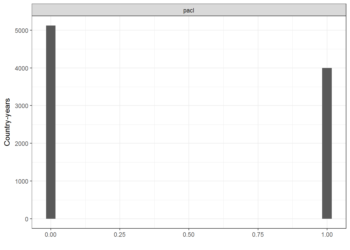
| pacl | 196 | 63 | 1946 | 2008 | 1981.94 | 2 | 0.44 | 0.00 | 0.00 | 1.00 | 0.50 |
| pacl_pmm | 196 | 63 | 1946 | 2008 | 1982.01 | 2 | 0.44 | 0.00 | 0.00 | 1.00 | 0.50 |
| PEPS1i | 175 | 204 | 1800 | 2003 | 1949.74 | 726 | -3.20 | -7.00 | -10.00 | 10.00 | 6.57 |
| PEPS1q | 176 | 204 | 1800 | 2003 | 1950.37 | 727 | -3.18 | -6.24 | -10.00 | 10.00 | 6.49 |
| PEPS1v | 177 | 204 | 1800 | 2003 | 1932.32 | 1866 | -2.87 | -4.00 | -10.00 | 10.00 | 5.66 |
| PEPS2i | 143 | 59 | 1945 | 2003 | 1981.28 | 843 | 3.72 | 5.00 | -9.59 | 10.00 | 4.39 |
| PEPS2q | 165 | 59 | 1945 | 2003 | 1978.99 | 856 | -1.13 | -1.46 | -10.00 | 10.00 | 6.91 |
| PEPS2v | 168 | 194 | 1810 | 2003 | 1937.77 | 2414 | -2.43 | -3.55 | -10.00 | 10.00 | 5.78 |
| pitf | 185 | 216 | 1800 | 2015 | 1939.20 | 5 | 2.42 | 2.00 | 1.00 | 5.00 | 1.48 |
| pitf_binary | 185 | 216 | 1800 | 2015 | 1939.20 | 2 | 1.36 | 1.00 | 1.00 | 2.00 | 0.48 |
| polcomp | 186 | 216 | 1800 | 2015 | 1939.20 | 13 | 1.30 | 6.00 | -88.00 | 10.00 | 17.76 |
| polity | 186 | 216 | 1800 | 2015 | 1938.89 | 24 | -4.08 | -3.00 | -88.00 | 10.00 | 17.67 |
| polity_pmm | 167 | 63 | 1946 | 2008 | 1980.85 | 21 | 0.13 | -1.00 | -10.00 | 10.00 | 7.50 |
| polity2 | 186 | 216 | 1800 | 2015 | 1938.91 | 21 | -0.60 | -3.00 | -10.00 | 10.00 | 7.07 |
| Polity3 | 181 | 204 | 1800 | 2003 | 1929.05 | 21 | -1.13 | -3.00 | -10.00 | 10.00 | 7.05 |
| polyarchy_contestation | 196 | 2 | 1985 | 2000 | 1993.11 | 9 | 5.82 | 6.00 | 1.00 | 9.00 | 2.90 |
| polyarchy_pmm | 194 | 2 | 1985 | 2000 | 1993.12 | 11 | 6.33 | 7.00 | 0.00 | 10.00 | 3.51 |
| polyarchy_reversed | 196 | 2 | 1985 | 2000 | 1993.11 | 11 | 6.35 | 7.00 | 0.00 | 10.00 | 3.52 |
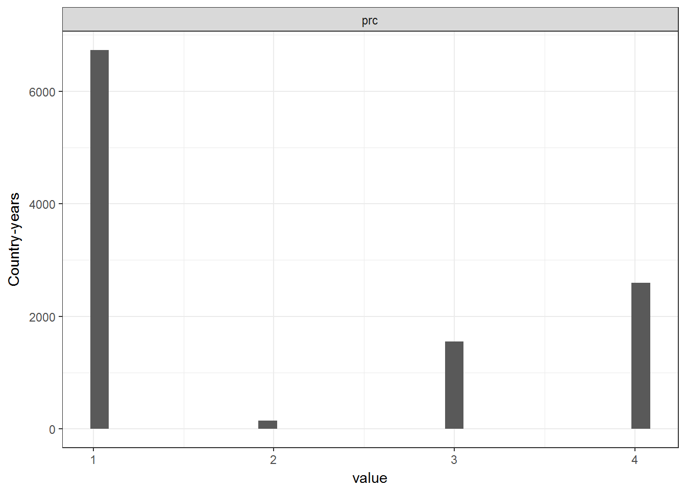
| prc | 149 | 252 | 1747 | 1998 | 1937.00 | 4 | 2.00 | 1.00 | 1.00 | 4.00 | 1.30 |
| prc_notrans | 149 | 252 | 1747 | 1998 | 1936.50 | 3 | 2.00 | 1.00 | 1.00 | 4.00 | 1.31 |
| prc_pmm | 148 | 53 | 1946 | 1998 | 1974.83 | 4 | 2.15 | 1.00 | 1.00 | 4.00 | 1.37 |
| przeworski | 197 | 221 | 1788 | 2008 | 1950.24 | 4 | 1.79 | 2.00 | 0.00 | 3.00 | 0.81 |
| svolik | 198 | 88 | 1921 | 2008 | 1980.99 | 2 | 1.44 | 1.00 | 1.00 | 2.00 | 0.50 |
| ulfelder | 167 | 56 | 1955 | 2010 | 1984.84 | 2 | 0.41 | 0.00 | 0.00 | 1.00 | 0.49 |
| utip_dichotomous | 152 | 44 | 1963 | 2006 | 1984.47 | 2 | 0.52 | 1.00 | 0.00 | 1.00 | 0.50 |
| utip_dichotomous_strict | 152 | 44 | 1963 | 2006 | 1984.47 | 2 | 0.48 | 0.00 | 0.00 | 1.00 | 0.50 |
| utip_trichotomous | 152 | 44 | 1963 | 2006 | 1984.47 | 3 | 0.99 | 1.00 | 0.00 | 2.00 | 0.98 |
| v2x_api | 173 | 116 | 1900 | 2015 | 1960.74 | 9320 | 0.47 | 0.41 | 0.02 | 0.98 | 0.31 |
| v2x_delibdem | 172 | 116 | 1900 | 2015 | 1960.75 | 9884 | 0.21 | 0.07 | 0.00 | 0.93 | 0.27 |
| v2x_egaldem | 173 | 116 | 1900 | 2015 | 1960.74 | 10212 | 0.25 | 0.15 | 0.01 | 0.92 | 0.25 |
| v2x_libdem | 173 | 116 | 1900 | 2015 | 1960.74 | 10662 | 0.26 | 0.15 | 0.01 | 0.93 | 0.25 |
| v2x_mpi | 173 | 116 | 1900 | 2015 | 1960.74 | 6114 | 0.18 | 0.00 | 0.00 | 0.93 | 0.28 |
| v2x_partipdem | 173 | 116 | 1900 | 2015 | 1960.72 | 9949 | 0.20 | 0.11 | 0.00 | 0.84 | 0.21 |
| v2x_polyarchy | 173 | 116 | 1900 | 2015 | 1960.74 | 9320 | 0.32 | 0.21 | 0.01 | 0.96 | 0.28 |
| vanhanen_competition | 193 | 203 | 1810 | 2012 | 1947.43 | 694 | 25.22 | 20.00 | 0.00 | 70.00 | 25.17 |
| vanhanen_democratization | 193 | 203 | 1810 | 2012 | 1947.43 | 445 | 8.43 | 1.10 | 0.00 | 49.00 | 11.68 |
| vanhanen_participation | 193 | 203 | 1810 | 2012 | 1947.43 | 760 | 21.10 | 14.00 | 0.00 | 71.00 | 21.88 |
| vanhanen_pmm | 192 | 63 | 1946 | 2008 | 1981.71 | 439 | 11.31 | 5.90 | 0.00 | 49.00 | 12.67 |
| wahman_teorell_hadenius | 193 | 39 | 1972 | 2010 | 1991.93 | 2 | 0.42 | 0.00 | 0.00 | 1.00 | 0.49 |
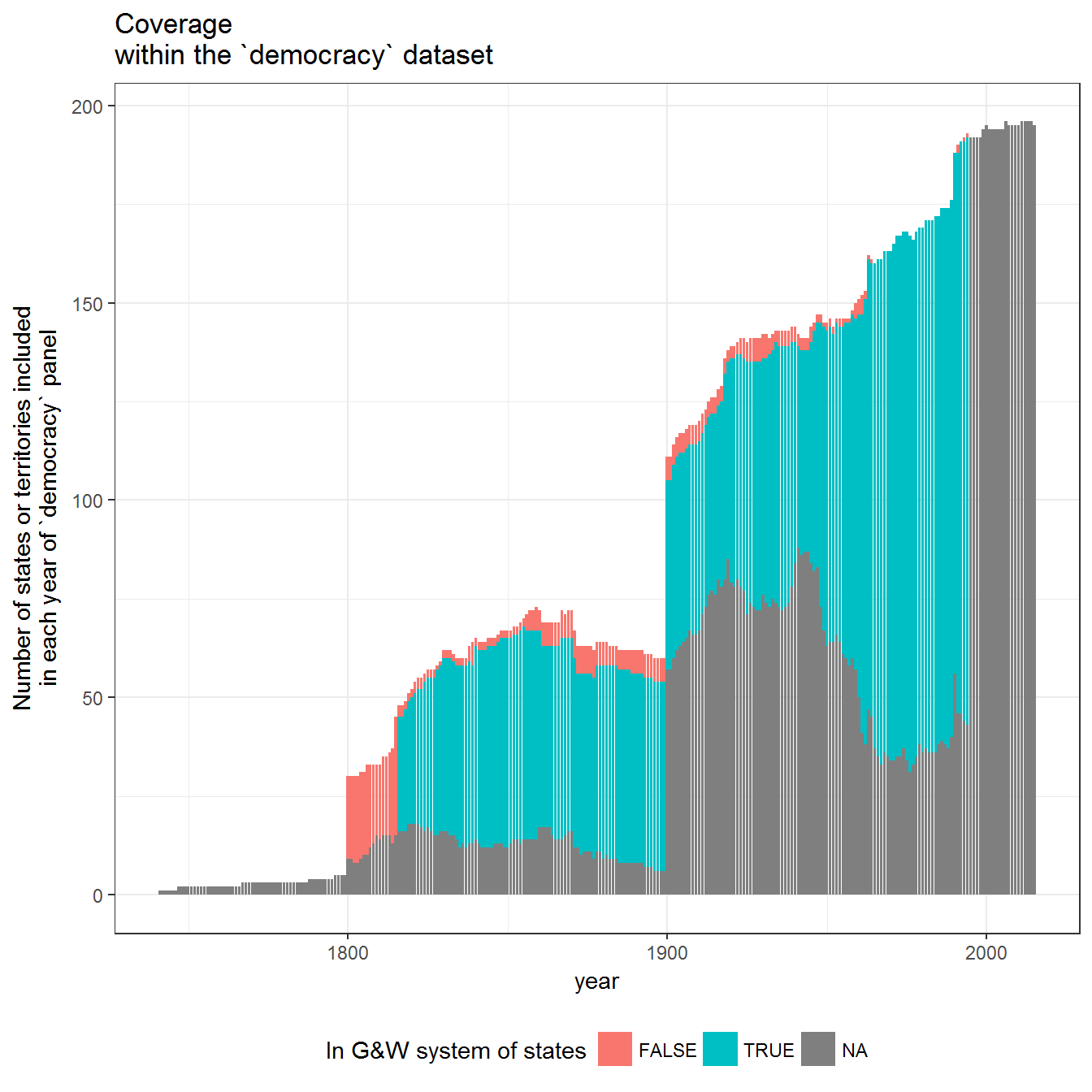
This is the dataset described in Arat 1991; the actual values are taken from Pemstein, Meserve, and Melton 2013 (the replication data for Pemstein, Meserve, and Melton 2010).
library(ggplot2)
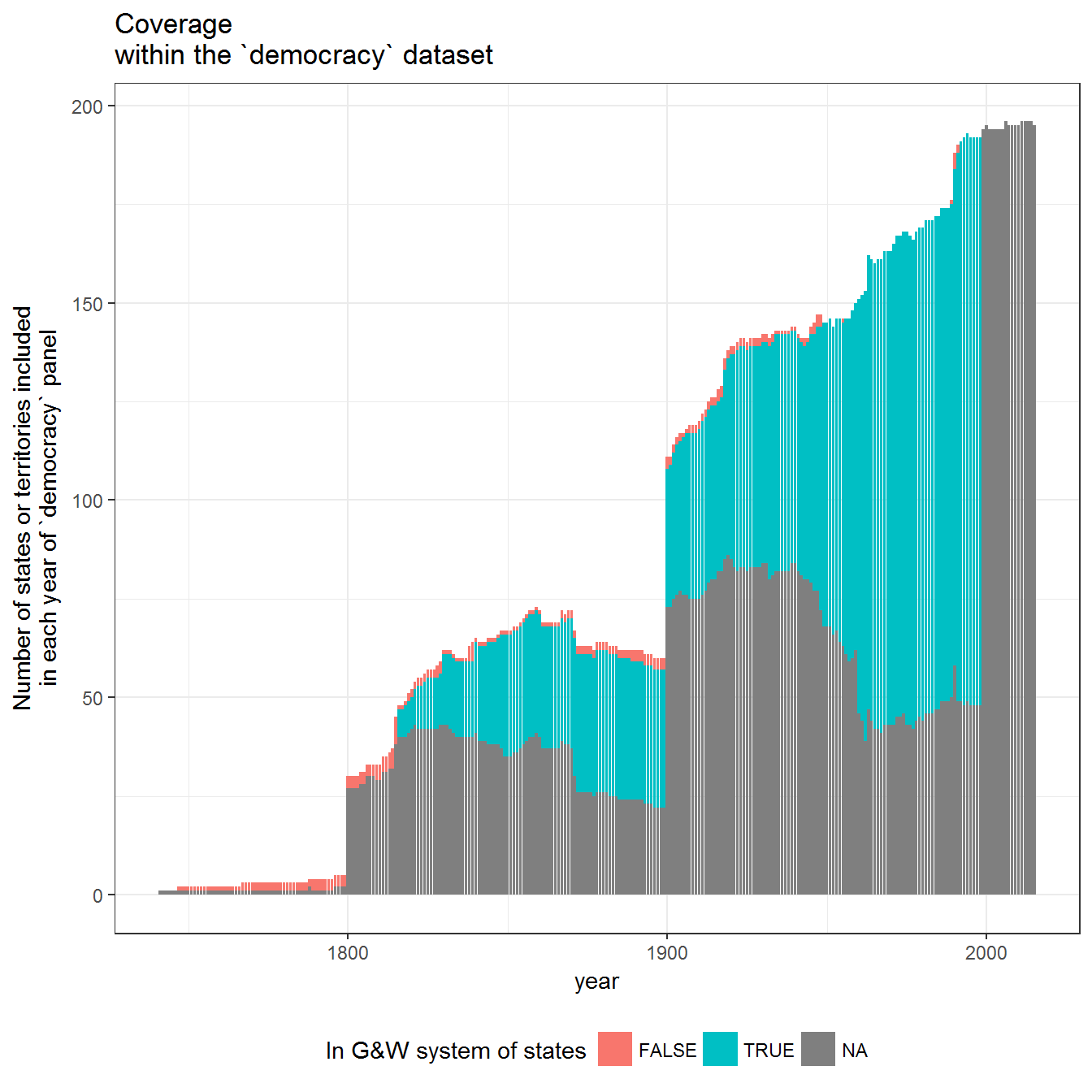
panel <- democracy %>% select(country_name,year) %>% distinct()
temporal_coverage <- function(data) {
data <- left_join(panel,data)
data <- data %>%
group_by(year, add=TRUE) %>%
count(year,in_system)
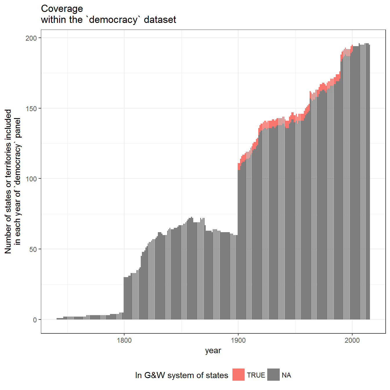
ggplot(data = data, aes(x=year,fill = in_system, y = n)) +
geom_bar(stat = "identity") +
theme_bw() +
theme(legend.position = "bottom") +
labs(fill = "In G&W system of states",
y = "Number of states or territories included\nin each year of `democracy` panel") +
ggtitle("Coverage \nwithin the `democracy` dataset")
}
library(rworldmap)
world <- getMap()
world <- fortify(world)## Regions defined for each Polygonsspatial_coverage <- function(data) {
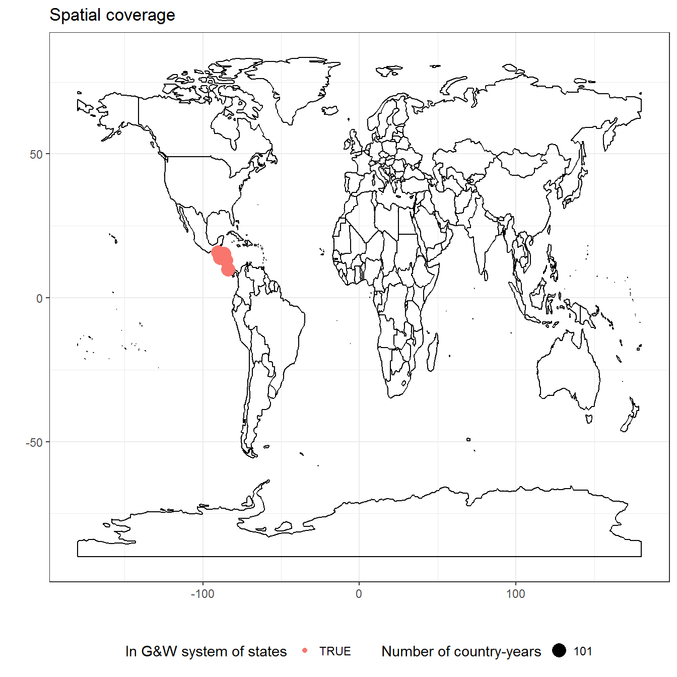
ggplot() +
geom_path(data = world, aes(x=long,y=lat,group=group)) +
theme_bw() +
theme(legend.position = "bottom") +
geom_count(data = data, aes(x=lon,y=lat,color = in_system)) +
labs(color = "In G&W system of states", y = "", x = "", size = "Number of country-years") +
ggtitle("Spatial coverage")
}
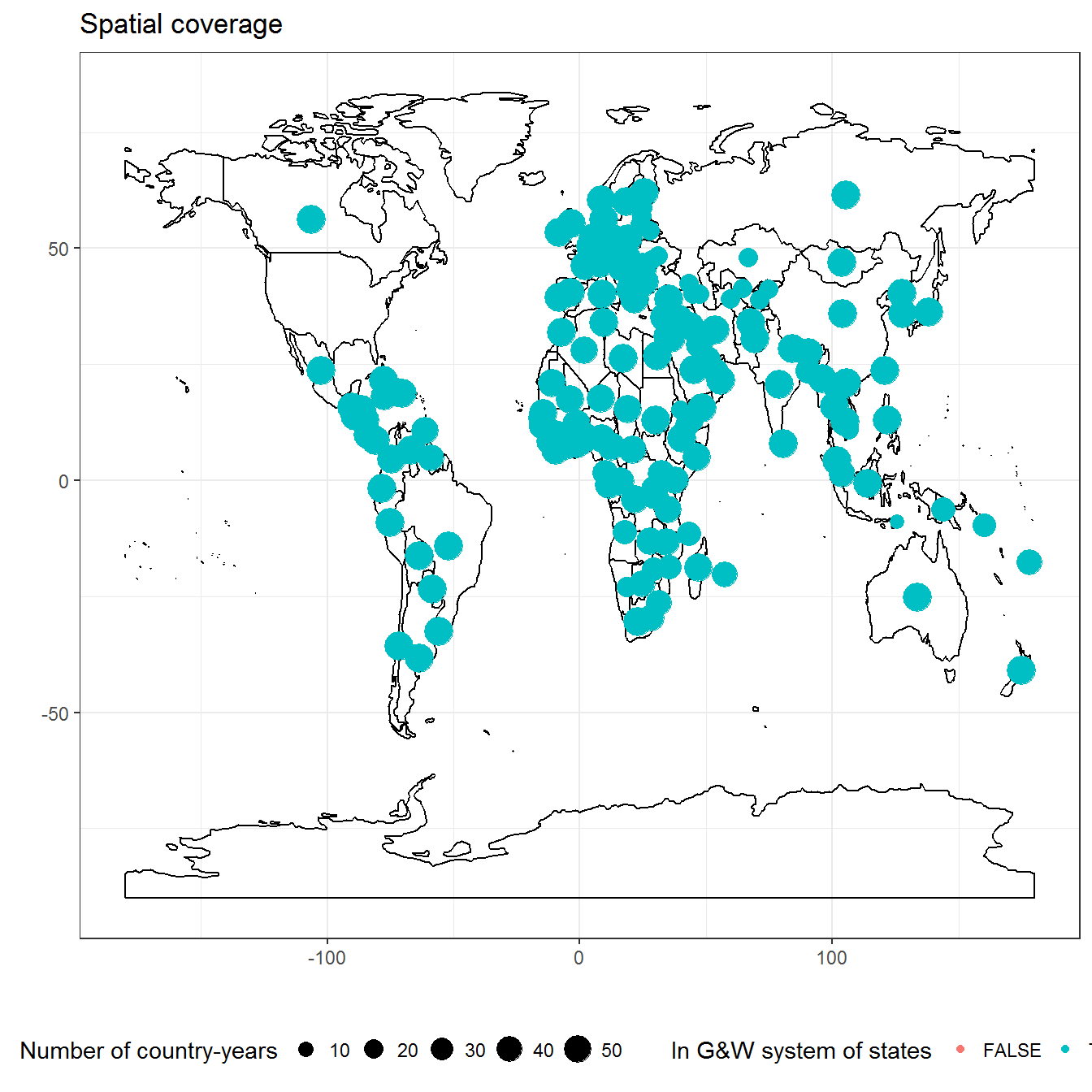
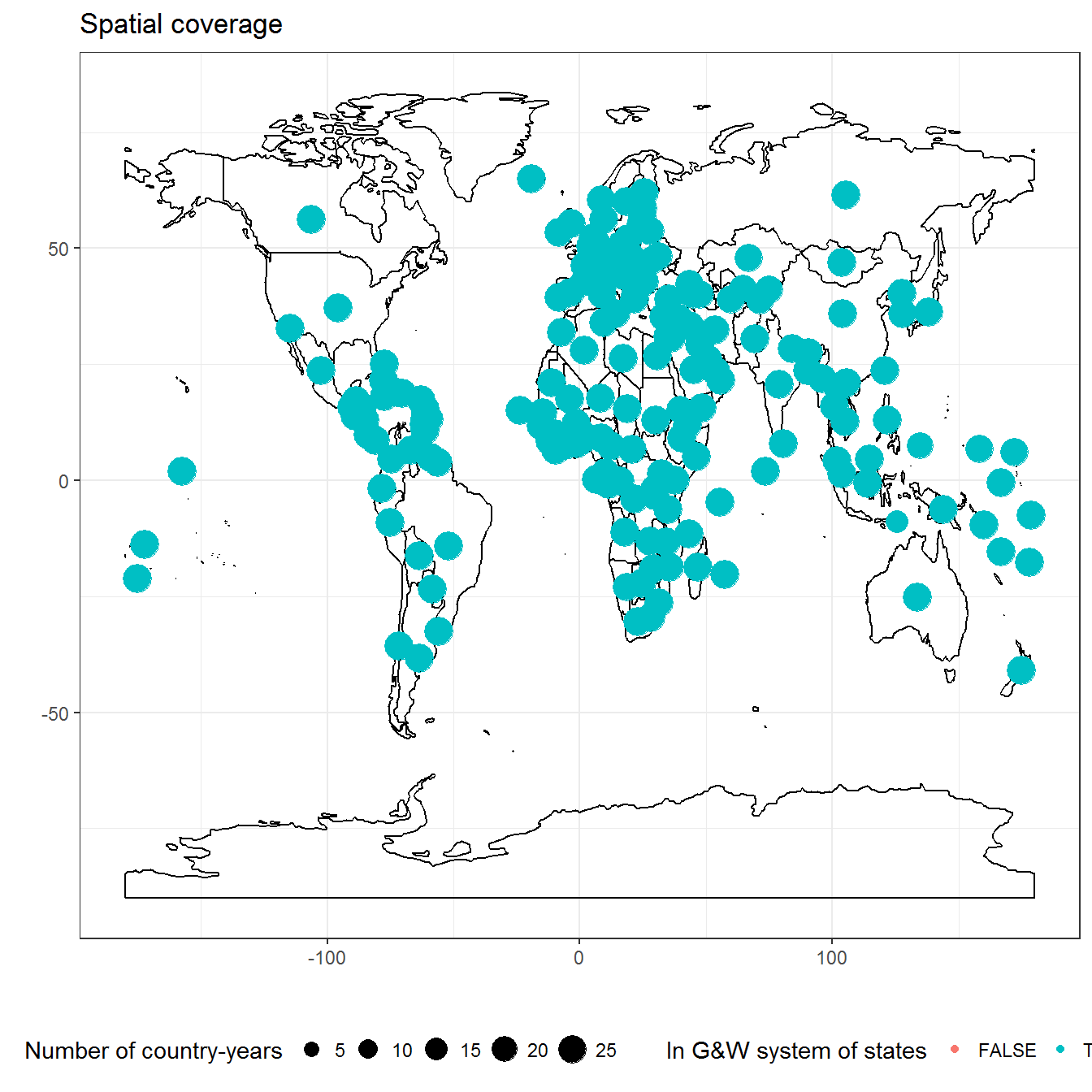
data <- democracy_long %>%
filter(variable == "arat_pmm")
temporal_coverage(data)## Joining, by = c("country_name", "year")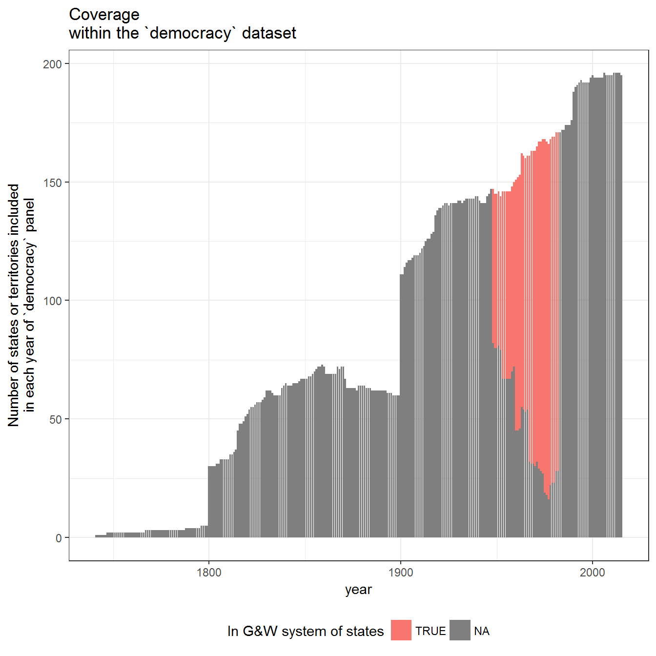
spatial_coverage(data)
ggplot(data = data) +
  geom_histogram(aes(x=value),bins=20) +
  theme_bw() +
  theme(legend.position = "bottom") +
  labs(y = "Country-years") +
  facet_wrap(~variable, ncol=2)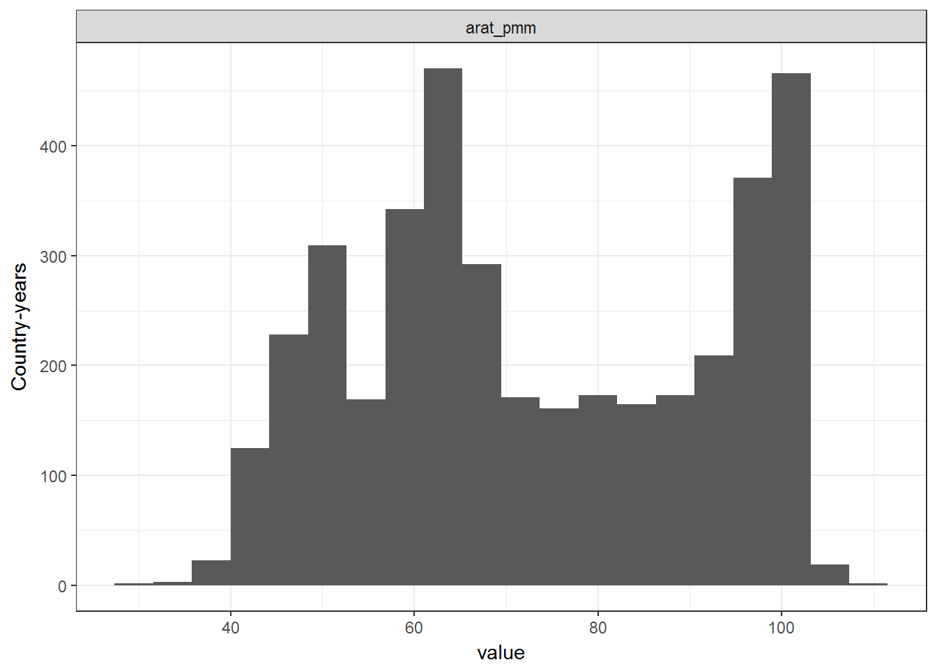
ggplot(data = data) +
  geom_density(aes(x=value)) +
  theme_bw() +
  theme(legend.position = "bottom") +
  labs(y = "Density") +
  facet_wrap(~variable, ncol=2)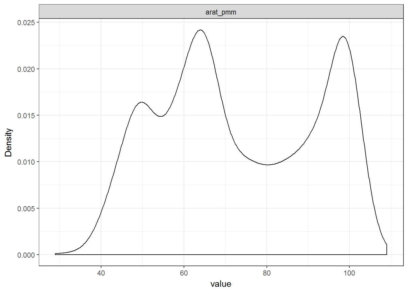
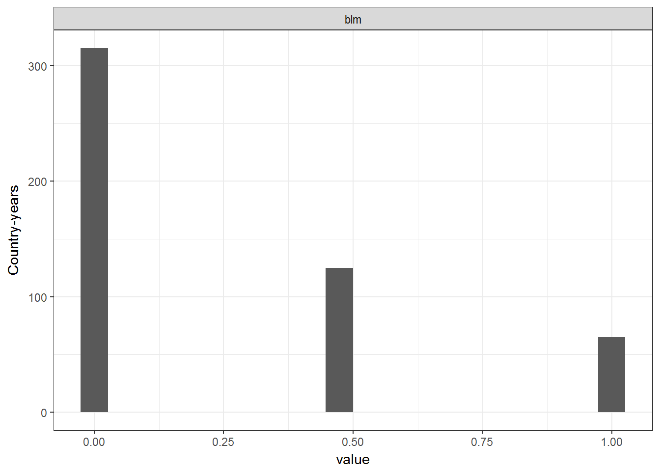
This is the dataset described in Bowman, Lehoucq, and Mahoney 2005.
This is the dataset described in Boix, Miller, and Rosato 2012.
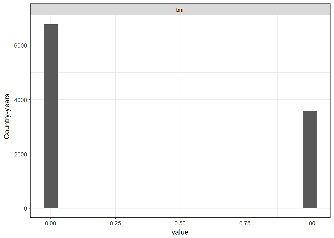
This is the dataset described in Bernhardt, Nordstrom, and Reenock 2001. The original dataset only counts periods of democracy in the period 1913-2005, since it is designed for event history analysis. To put it in country-year format, this package assumes that country-years in independent states between 1913 and 2005 are to be counted as non-democratic if they are not explicitly said to be democratic by BNR. (Country-years are considered to be independent if the state is not a microstate and appears in Gleditasch and Ward’s [1999] panel of indepdent states for the period).
This is the dataset described in Bollen 2001. The actual values are taken from Pemstein, Meserve, and Melton’s replication data for their article (Pemstein, Meserve, and Melton 2013).
data <- democracy_long %>% filter(variable == "bollen_pmm")
temporal_coverage(data)## Joining, by = c("country_name", "year")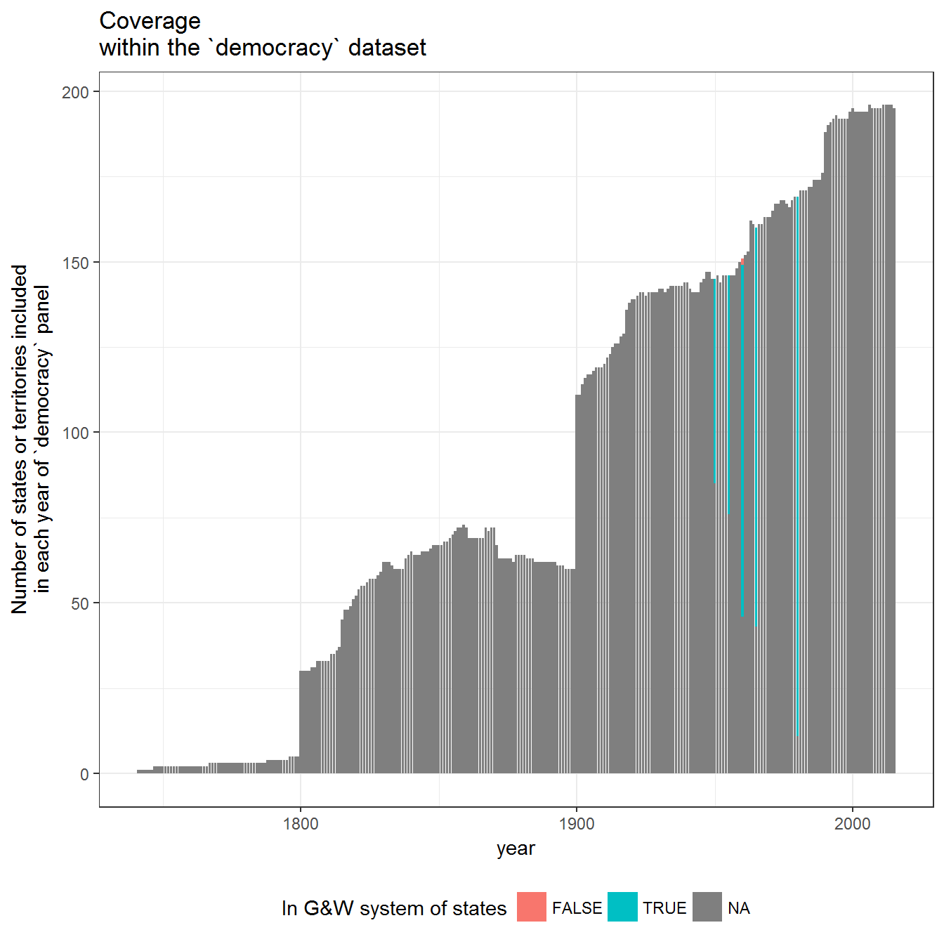
spatial_coverage(data)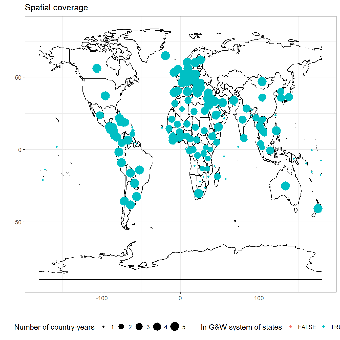
ggplot(data = data) +
  geom_histogram(aes(x=value),bins=20) +
  theme_bw() +
  theme(legend.position = "bottom") +
  labs(y = "Country-years") +
  facet_wrap(~variable, ncol=2)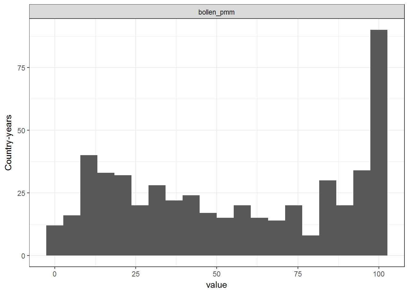
ggplot(data = data) +
geom_density(aes(x=value)) +
theme_bw() +
theme(legend.position = "bottom") +
labs(y = "Density") +
facet_wrap(~variable, ncol=2)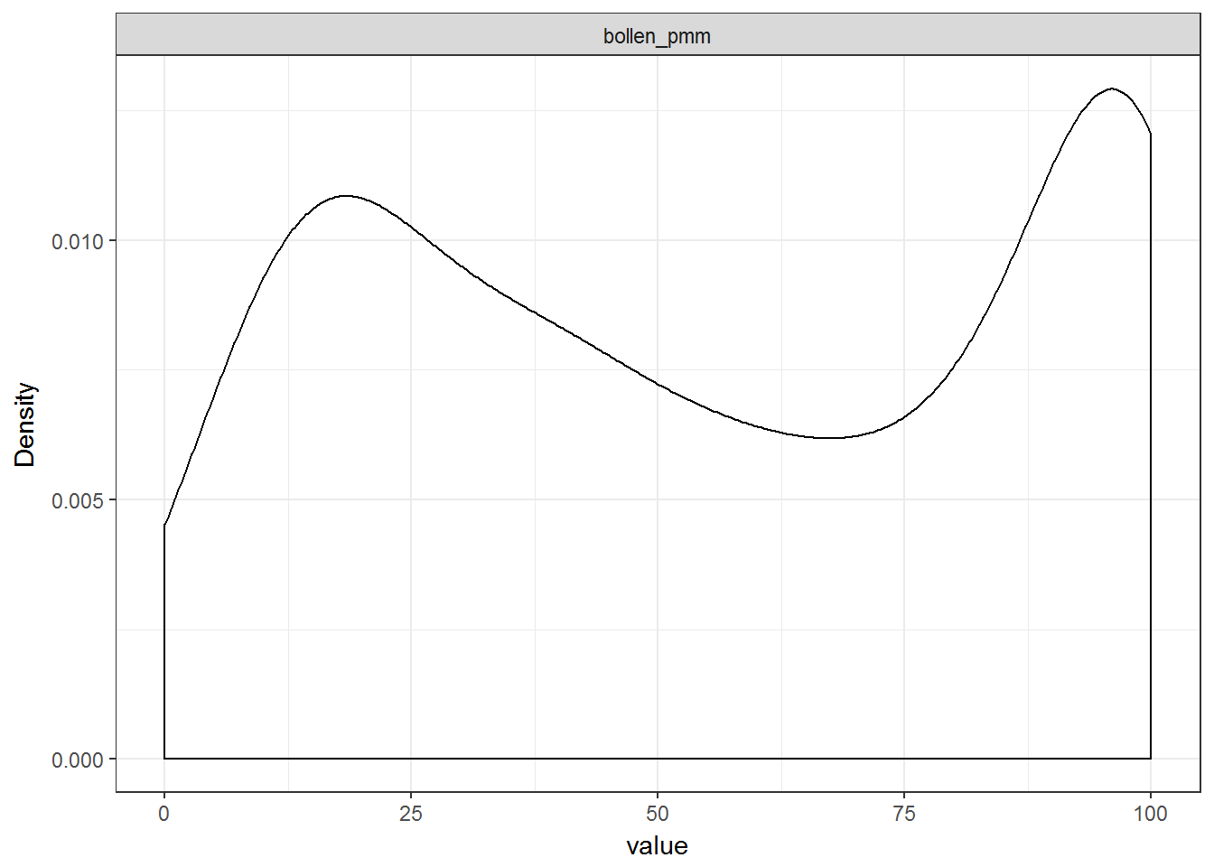
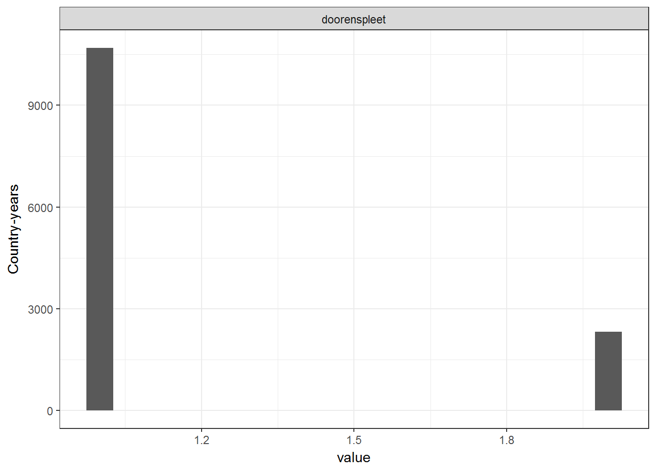
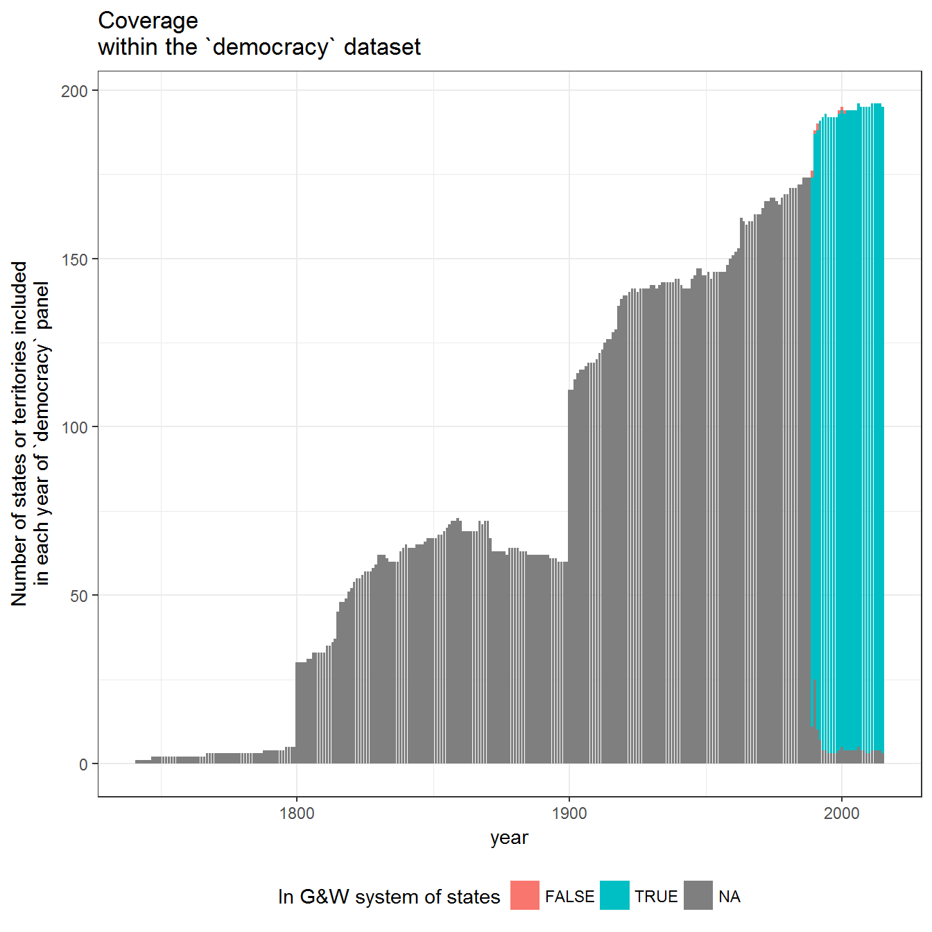
This is the dataset described in Doorenspleet 2000.
This contains the Economist Intelligence Unit’s index of democracy (EIU 2012). The actual data is taken from the World Bank’s Governance Indicators (http://www.govindicators.org)
data <- democracy_long %>% filter(variable == "eiu")
temporal_coverage(data)## Joining, by = c("country_name", "year")
spatial_coverage(data)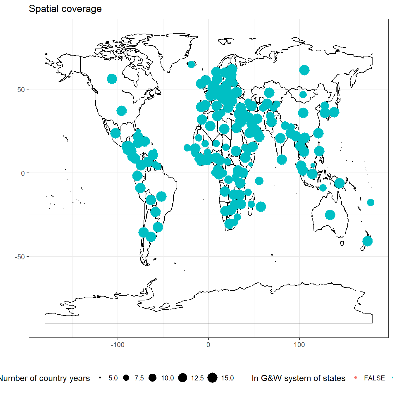
ggplot(data = data) +
  geom_histogram(aes(x=value),bins=20) +
  theme_bw() +
  theme(legend.position = "bottom") +
  labs(y = "Country-years") +
  facet_wrap(~variable, ncol=2)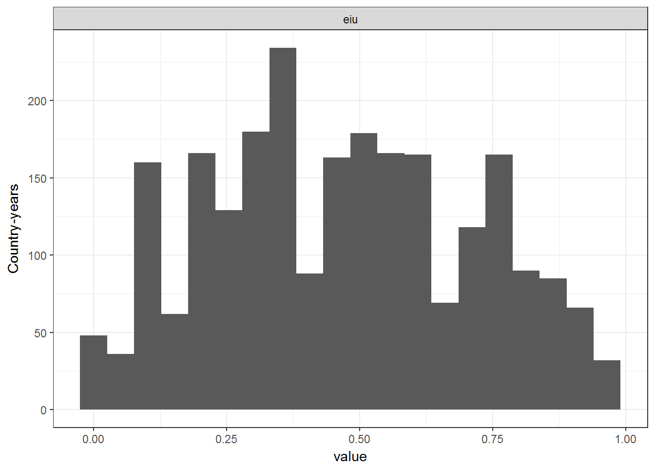
ggplot(data = data) +
geom_density(aes(x=value)) +
theme_bw() +
theme(legend.position = "bottom") +
labs(y = "Density") +
facet_wrap(~variable, ncol=2)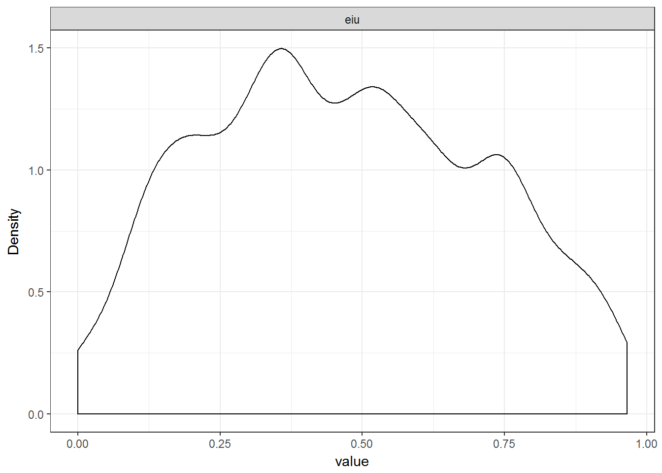
This is the Freedom in the World Index, to 2015 (Freedom House 2016). Some non-independent territories have been excluded from the original data.
data <- democracy_long %>% filter(variable %in% c("freedomhouse"))
temporal_coverage(data)## Joining, by = c("country_name", "year")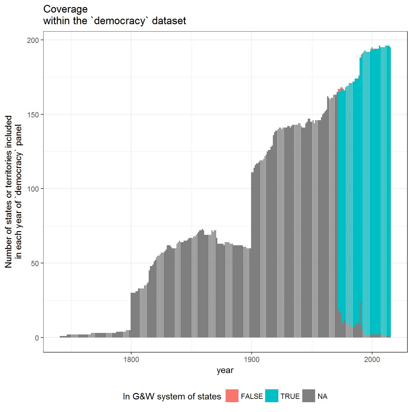
spatial_coverage(data)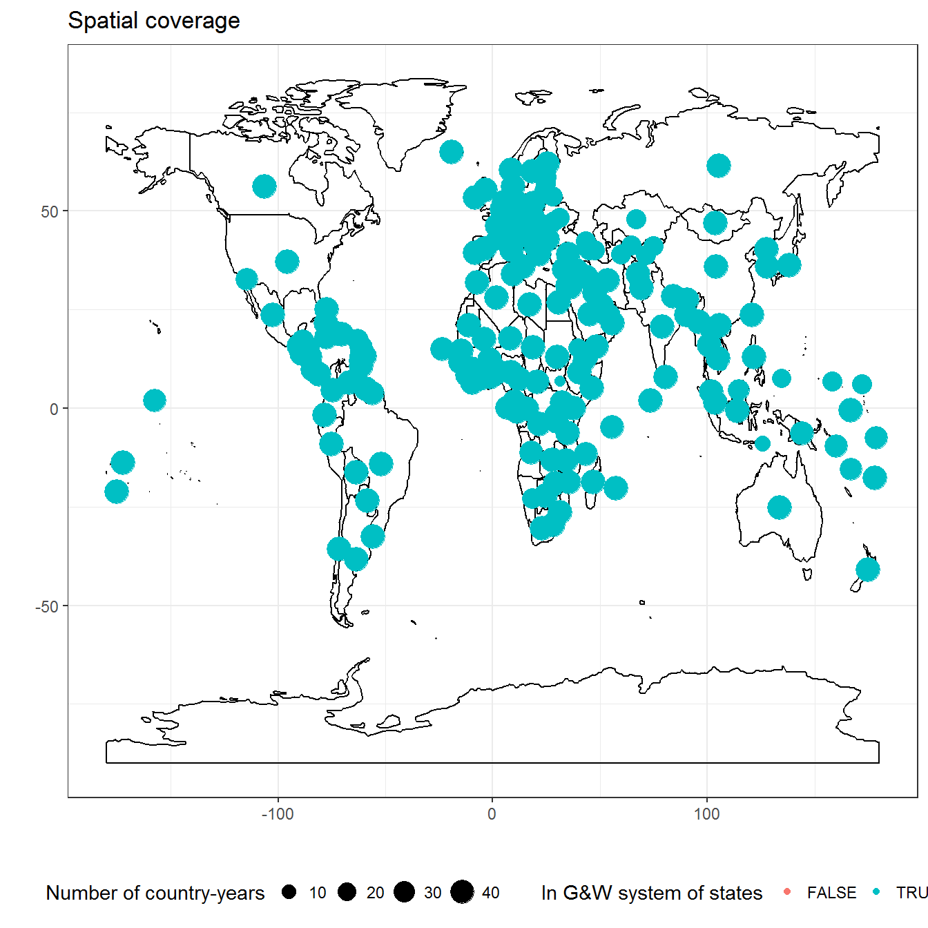
ggplot(data = data) +
  geom_histogram(aes(x=value),bins=20) +
  theme_bw() +
  theme(legend.position = "bottom") +
  labs(y = "Country-years") +
  facet_wrap(~variable, ncol=2)
ggplot(data = data) +
  geom_density(aes(x=value)) +
  theme_bw() +
  theme(legend.position = "bottom") +
  labs(y = "Density") +
  facet_wrap(~variable, ncol=2)
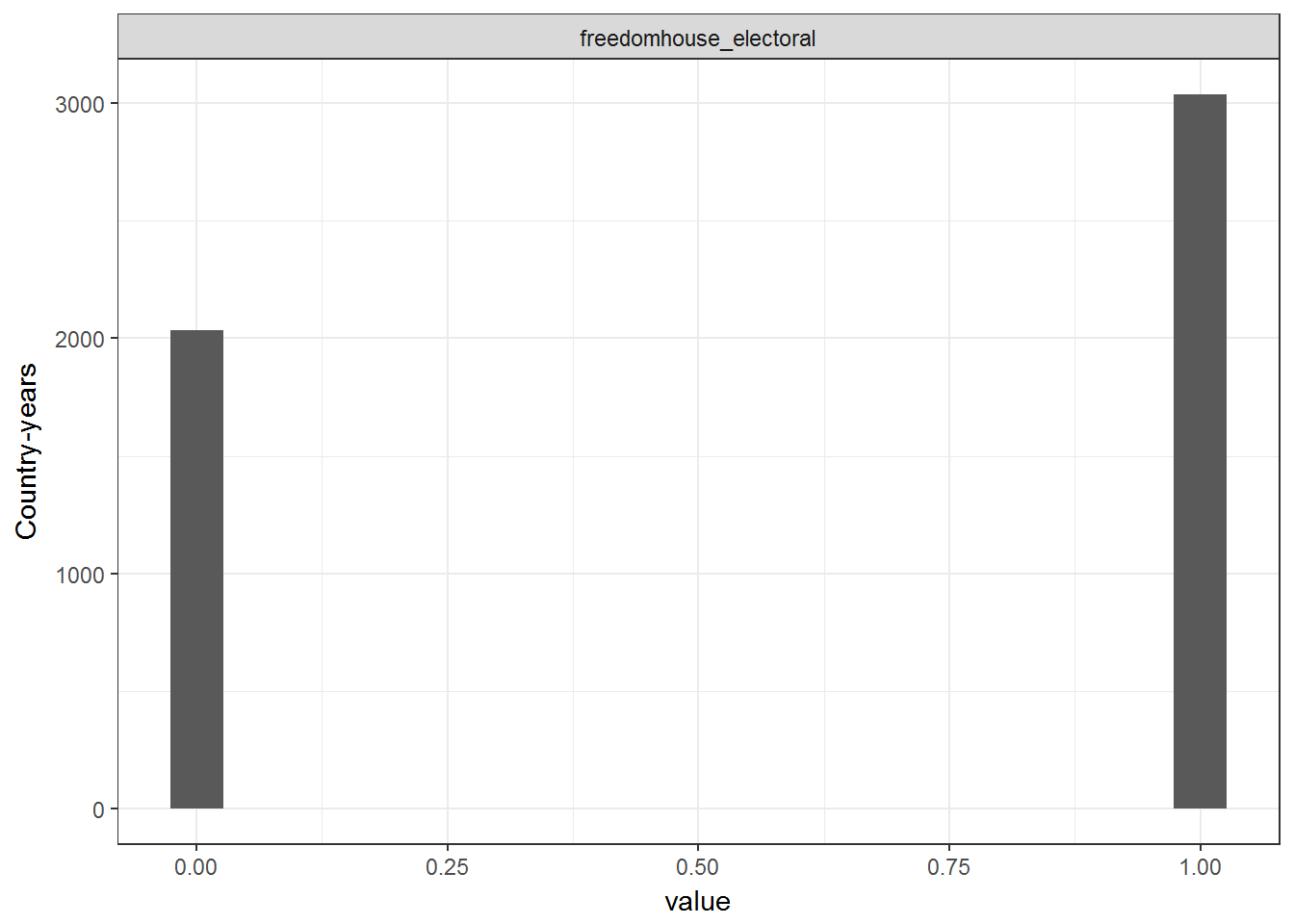
This is Freedom House’s list of electoral democracies, to 2015 (Freedom House 2016). Some non-independent territories have been excluded from the original data.
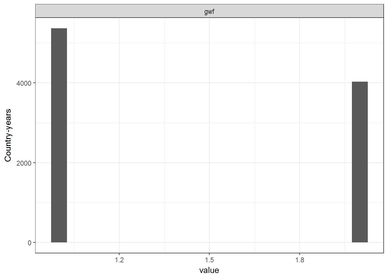
This is a measure of democracy/non-democracy derived from the dataset described in Geddes, Wright, and Frantz 2014. The original data has been extended beyond 1945 by reconciling the information contained in the original dataset’s gwf_startdate, gwf_spell, and gwf_casename variables, which encode the start year of each democratic and non-democratic regime (sometimes going back to the 18th century).
This is the dataset in Hadenius 1992. Actual values taken from Pemstein, Meserve, and Melton 2013.
data <- democracy_long %>% filter(variable == "hadenius_pmm")
temporal_coverage(data) ## Joining, by = c("country_name", "year")
spatial_coverage(data)
ggplot(data = data) +
  geom_histogram(aes(x=value),bins=20) +
  theme_bw() +
  theme(legend.position = "bottom") +
  labs(y = "Country-years") +
  facet_wrap(~variable, ncol=2)
ggplot(data = data) +
  geom_density(aes(x=value)) +
  theme_bw() +
  theme(legend.position = "bottom") +
  labs(y = "Density") +
  facet_wrap(~variable, ncol=2)
The dataset described in Kailitz 2013.
data <- democracy_long %>% filter(variable == "kailitz_binary")
temporal_coverage(data)## Joining, by = c("country_name", "year")
spatial_coverage(data)
data <- democracy_long %>% filter(variable %in% c("kailitz_binary","kailitz_tri"))
ggplot(data = data) +
geom_histogram(aes(x=value)) +
theme_bw() +
theme(legend.position = "bottom") +
labs(y = "Country-years") +
facet_wrap(~variable, ncol=2)## `stat_bin()` using `bins = 30`. Pick better value with `binwidth`.
Note that 316 of the country-years in the Kailitz dataset are classified with more than one regime type.
kable(kailitz_yearly %>%
count(multiple_regimes = grepl("-",combined_regime)))| multiple_regimes | n |
|---|---|
| FALSE | 9290 |
| TRUE | 316 |
kable(kailitz_yearly %>%
filter(grepl("-",combined_regime)) %>%
group_by(country_name) %>%
arrange(country_name,year) %>%
group_by(combined_regime, add=TRUE) %>%
summarise(min = min(year), max = max(year), n = n()))| country_name | combined_regime | min | max | n |
|---|---|---|---|---|
| Afghanistan | Electoral Autocracy-Personalist Autocracy | 2010 | 2010 | 1 |
| Algeria | Electoral Autocracy-One party Autocracy | 1989 | 1991 | 3 |
| Angola | Electoral Autocracy-State Failure or Occupation | 2010 | 2010 | 1 |
| Benin | Electoral Autocracy-Personalist Autocracy | 1960 | 1962 | 3 |
| Benin | Military Autocracy-Personalist Autocracy | 1965 | 1974 | 8 |
| Benin | Personalist Autocracy-Transition | 1963 | 1971 | 4 |
| Burundi | Electoral Autocracy-State Failure or Occupation | 1993 | 1995 | 3 |
| Burundi | One party Autocracy-Personalist Autocracy | 1982 | 1983 | 2 |
| Cambodia (Kampuchea) | Communist Ideocracy-State Failure or Occupation | 1981 | 1990 | 10 |
| Central African Republic | Electoral Autocracy-One party Autocracy | 1991 | 1992 | 2 |
| Colombia | Electoral Autocracy-Liberal Democracy | 1946 | 1947 | 2 |
| Colombia | State Failure or Occupation-Transition | 1948 | 1952 | 5 |
| Cuba | Electoral Autocracy-Liberal Democracy | 1946 | 1951 | 6 |
| Ecuador | Electoral Autocracy-Personalist Autocracy | 1970 | 1971 | 2 |
| Ecuador | Electoral Autocracy-Transition | 2000 | 2001 | 2 |
| Guinea-Bissau | Military Autocracy-Personalist Autocracy | 1980 | 1983 | 4 |
| Guinea-Bissau | Military Autocracy-Transition | 2004 | 2004 | 1 |
| Haiti | Electoral Autocracy-Transition | 1946 | 1947 | 2 |
| Honduras | Electoral Autocracy-Liberal Democracy | 1957 | 1962 | 6 |
| Indonesia | Personalist Autocracy-Transition | 1952 | 1967 | 12 |
| Kuwait | Monarchy-State Failure or Occupation | 1990 | 1990 | 1 |
| Lebanon | State Failure or Occupation-Transition | 2000 | 2001 | 2 |
| Lesotho | Electoral Autocracy-State Failure or Occupation | 1998 | 1999 | 2 |
| Lesotho | Electoral Autocracy-Transition | 2000 | 2001 | 2 |
| Liberia | Personalist Autocracy-State Failure or Occupation | 1990 | 1990 | 1 |
| Madagascar (Malagasy) | Military Autocracy-Personalist Autocracy | 1972 | 1974 | 3 |
| Madagascar (Malagasy) | Personalist Autocracy-Transition | 1975 | 1975 | 1 |
| Mauritania | Electoral Autocracy-Military Autocracy | 2008 | 2008 | 1 |
| Mozambique | Personalist Autocracy-Transition | 1991 | 1993 | 3 |
| Nicaragua | Communist Ideocracy-Electoral Autocracy | 1984 | 1989 | 6 |
| Nicaragua | Communist Ideocracy-State Failure or Occupation | 1980 | 1981 | 2 |
| Nicaragua | Communist Ideocracy-Transition | 1982 | 1983 | 2 |
| Nicaragua | Electoral Autocracy-Personalist Autocracy | 1972 | 1972 | 1 |
| Nicaragua | Military Autocracy-Personalist Autocracy | 1973 | 1973 | 1 |
| Niger | Electoral Autocracy-Liberal Democracy | 2000 | 2010 | 11 |
| Peru | Electoral Autocracy-Liberal Democracy | 1963 | 1967 | 5 |
| Philippines | Electoral Autocracy-Liberal Democracy | 1946 | 1971 | 26 |
| Philippines | Liberal Democracy-Personalist Autocracy | 1994 | 2002 | 9 |
| Portugal | Military Autocracy-Transition | 1974 | 1975 | 2 |
| Seychelles | Electoral Autocracy-Liberal Democracy | 2007 | 2010 | 4 |
| Seychelles | Liberal Democracy-Transition | 1976 | 1976 | 1 |
| Somalia | Liberal Democracy-Transition | 1960 | 1968 | 9 |
| Somalia | Military Autocracy-Personalist Autocracy | 1969 | 1990 | 22 |
| Somalia | Military Autocracy-State Failure or Occupation | 1991 | 1991 | 1 |
| Spain | Military Autocracy-One party Autocracy-Personalist Autocracy | 1946 | 1974 | 29 |
| Sri Lanka (Ceylon) | Electoral Autocracy-Liberal Democracy | 1960 | 2010 | 51 |
| Sri Lanka (Ceylon) | Electoral Autocracy-Transition | 1948 | 1959 | 12 |
| Syria | One party Autocracy-Personalist Autocracy | 2000 | 2010 | 11 |
| Tunisia | One party Autocracy-Personalist Autocracy | 1975 | 1978 | 4 |
| Venezuela | Military Autocracy-Personalist Autocracy | 1948 | 1957 | 10 |
| Yemen (Arab Republic of Yemen) | Monarchy-Transition | 1946 | 1947 | 2 |
The following are especially troublesome, since the multiple categories do not make sense:
kable(kailitz_yearly %>%
filter(grepl("-",combined_regime)) %>%
group_by(country_name) %>%
arrange(country_name,year) %>%
group_by(combined_regime, add=TRUE) %>%
summarise(min = min(year), max = max(year), n = n()) %>%
filter(grepl("democracy",combined_regime, ignore.case=TRUE)))| country_name | combined_regime | min | max | n |
|---|---|---|---|---|
| Colombia | Electoral Autocracy-Liberal Democracy | 1946 | 1947 | 2 |
| Cuba | Electoral Autocracy-Liberal Democracy | 1946 | 1951 | 6 |
| Honduras | Electoral Autocracy-Liberal Democracy | 1957 | 1962 | 6 |
| Niger | Electoral Autocracy-Liberal Democracy | 2000 | 2010 | 11 |
| Peru | Electoral Autocracy-Liberal Democracy | 1963 | 1967 | 5 |
| Philippines | Electoral Autocracy-Liberal Democracy | 1946 | 1971 | 26 |
| Philippines | Liberal Democracy-Personalist Autocracy | 1994 | 2002 | 9 |
| Seychelles | Electoral Autocracy-Liberal Democracy | 2007 | 2010 | 4 |
| Seychelles | Liberal Democracy-Transition | 1976 | 1976 | 1 |
| Somalia | Liberal Democracy-Transition | 1960 | 1968 | 9 |
| Sri Lanka (Ceylon) | Electoral Autocracy-Liberal Democracy | 1960 | 2010 | 51 |
I have constructed the index to classify a country as “democratic” only if it is not also classified as a non-democratic regime as well. Here are the index counts for each regime type:
kable(kailitz_yearly %>%
count(kailitz_binary,kailitz_tri,combined_regime))| kailitz_binary | kailitz_tri | combined_regime | n |
|---|---|---|---|
| 0 | 0 | Communist Ideocracy | 788 |
| 0 | 0 | Communist Ideocracy-Electoral Autocracy | 6 |
| 0 | 0 | Communist Ideocracy-State Failure or Occupation | 12 |
| 0 | 0 | Communist Ideocracy-Transition | 2 |
| 0 | 0 | Electoral Autocracy-Military Autocracy | 1 |
| 0 | 0 | Electoral Autocracy-One party Autocracy | 5 |
| 0 | 0 | Electoral Autocracy-Personalist Autocracy | 7 |
| 0 | 0 | Electoral Autocracy-State Failure or Occupation | 6 |
| 0 | 0 | Electoral Autocracy-Transition | 18 |
| 0 | 0 | Liberal Democracy-Personalist Autocracy | 9 |
| 0 | 0 | Liberal Democracy-Transition | 10 |
| 0 | 0 | Military Autocracy | 570 |
| 0 | 0 | Military Autocracy-One party Autocracy-Personalist Autocracy | 29 |
| 0 | 0 | Military Autocracy-Personalist Autocracy | 48 |
| 0 | 0 | Military Autocracy-State Failure or Occupation | 1 |
| 0 | 0 | Military Autocracy-Transition | 3 |
| 0 | 0 | Monarchy | 987 |
| 0 | 0 | Monarchy-State Failure or Occupation | 1 |
| 0 | 0 | Monarchy-Transition | 2 |
| 0 | 0 | One party Autocracy | 486 |
| 0 | 0 | One party Autocracy-Personalist Autocracy | 17 |
| 0 | 0 | Personalist Autocracy | 463 |
| 0 | 0 | Personalist Autocracy-State Failure or Occupation | 1 |
| 0 | 0 | Personalist Autocracy-Transition | 20 |
| 0 | 0 | State Failure or Occupation | 245 |
| 0 | 0 | State Failure or Occupation-Transition | 7 |
| 0 | 0 | Transition | 319 |
| 0 | 1 | Electoral Autocracy | 1477 |
| 0 | 1 | Electoral Autocracy-Liberal Democracy | 111 |
| 1 | 2 | Liberal Democracy | 3955 |
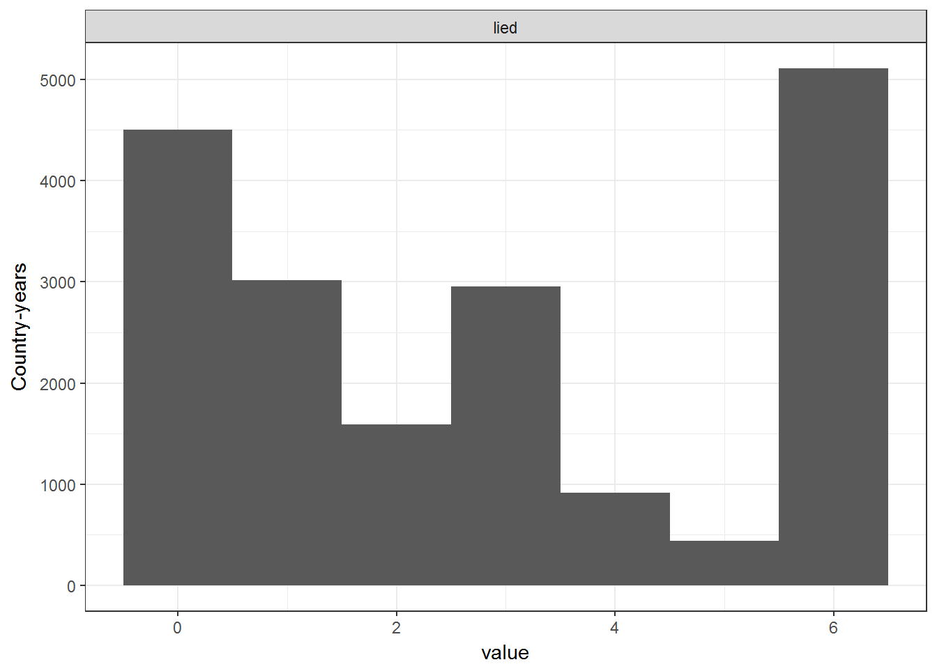
This is the Lexical Index of Democracy described in Skaaning, Gerring, and Bartusevicius 2015 (version 3, updated to 2015).
This is a measure of democracy derived from the authoritarian regimes dataset in Magaloni, Chu, and Min 2013. The original dataset has been extended beyond 1950 using the information encoded in the duration_nr variable of the original dataset, which provides information about the start date of each regime.
data <- democracy_long %>% filter(variable == "magaloni_democ_binary")
temporal_coverage(data) +
geom_vline(xintercept = 1950) +
annotate("text", label = "Limit of original dataset", x = 1950,y = 100, angle=90)## Joining, by = c("country_name", "year")
spatial_coverage(data)
One change has been made (Pakistan 1971/1972 appears to have been misclassified as a democracy).
Note magaloni_regime_tri identifies as “hybrid” (middle level) all multiparty autocracies.
data <- democracy_long %>% filter(variable %in% c("magaloni_democ_binary","magaloni_regime_tri"))
ggplot(data = data) +
geom_histogram(aes(x=value)) +
theme_bw() +
theme(legend.position = "bottom") +
labs(y = "Country-years") +
facet_wrap(~variable, ncol=2)## `stat_bin()` using `bins = 30`. Pick better value with `binwidth`.
This is the dataset in Mainwaring, Brinks, and Perez Linan 2008.
This is the dataset in Munck 2009. Taken from Pemstein, Meserve, and Melton 2013.
data <- democracy_long %>% filter(variable == "munck_pmm")
temporal_coverage(data) ## Joining, by = c("country_name", "year")
spatial_coverage(data)
ggplot(data = data) +
geom_histogram(aes(x=value)) +
theme_bw() +
theme(legend.position = "bottom") +
labs(y = "Country-years") +
facet_wrap(~variable, ncol=2)## `stat_bin()` using `bins = 30`. Pick better value with `binwidth`.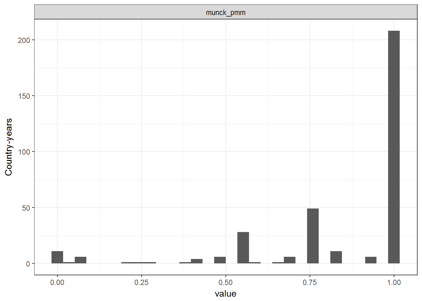
ggplot(data = data) +
  geom_density(aes(x=value)) +
  theme_bw() +
  theme(legend.position = "bottom") +
  labs(y = "Density") +
  facet_wrap(~variable, ncol=2)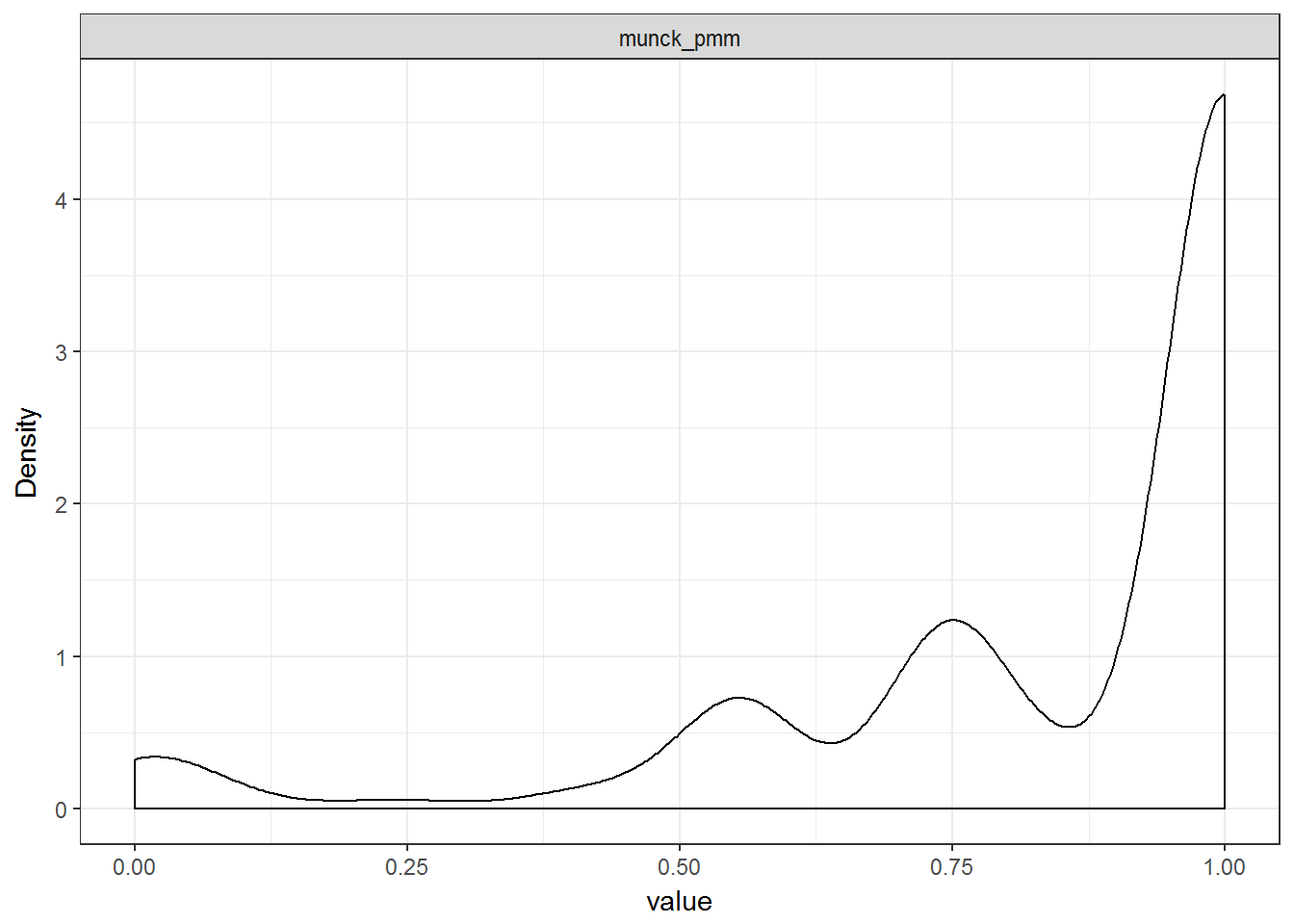
This is the dataset described in Cheibub, Gandhi, and Vreeland 2010.
This is the dataset described in Moon et al 2006.
The democracy file contains seven variables from this dataset: PEPS1i, PEPS2i, PEPS1q, PEPS2q, PEPS1v,PEPS2v, and Polity3, a cleaned up version of the polity2 variable in the Polity IV data. The PEPS* variables are constructed from Polity3 and a participation variable derived either from Vanhanen’s population and raw participation data (variables ending in *v) or from voting turnout data from IDEA (variables ending in q or i).
data <- democracy_long %>% filter(variable %in% c("PEPS1i","PEPS2i","PEPS1q","PEPS2q","PEPS1v","PEPS2v","Polity3"))
data <- left_join(panel,data) ## Joining, by = c("country_name", "year")data <- data %>% group_by(variable,year, add=TRUE) %>% count_(vars = c("year","in_system","variable"))
ggplot(data = data, aes(x=year,fill = in_system, y = n)) +
geom_bar(stat = "identity") +
theme_bw() +
theme(legend.position = "bottom") +
labs(fill = "In G&W system of states", y = "Number of states or territories\nin each year of `democracy` panel") +
ggtitle("Temporal coverage \nwithin the `democracy` dataset") +
facet_wrap(~variable) 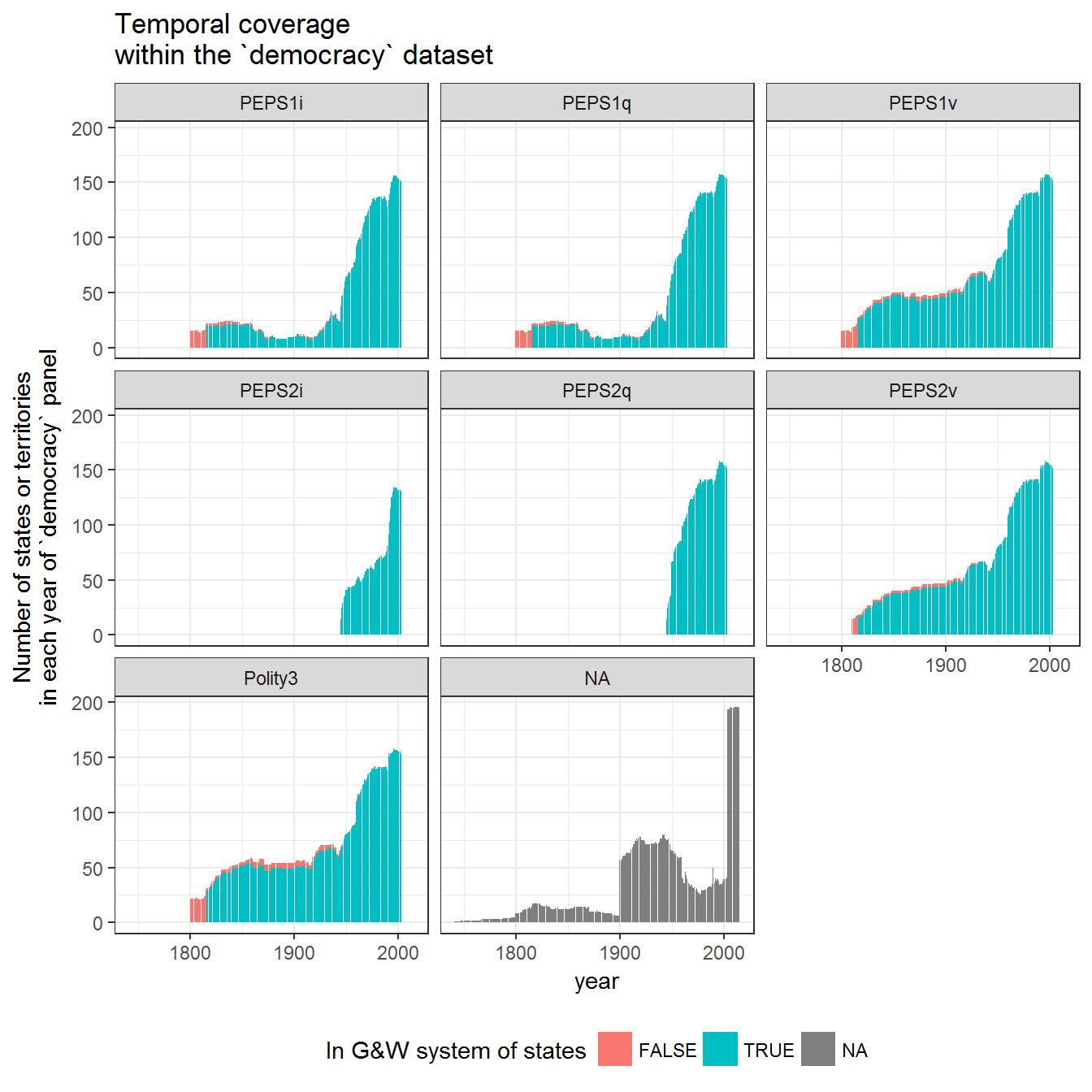
data <- democracy_long %>% filter(variable %in% c("PEPS1i","PEPS2i","PEPS1q","PEPS2q","PEPS1v","PEPS2v"))
spatial_coverage(data)
ggplot(data = data) +
geom_histogram(aes(x=value),binwidth=1) +
theme_bw() +
theme(legend.position = "bottom") +
labs(y = "Country-years", x="") +
facet_wrap(~variable, ncol=2)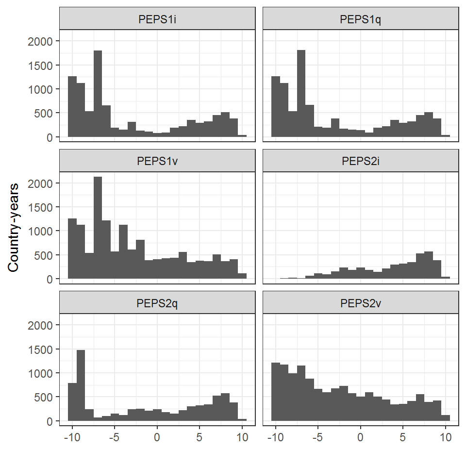
library(GGally)
ggcorr(data = democracy %>% select(PEPS1i:PEPS2v), label=TRUE,label_round=3) + scale_fill_gradient2(midpoint = 0.7)## Scale for 'fill' is already present. Adding another scale for 'fill',
## which will replace the existing scale.
The Polity3 variable is different from the polity2 variable in the following cases, mostly due to the different way in which Moon et al recode transitional periods, but in some cases due to revisions in the underlying Polity IV dataset since 2006:
kable(democracy %>%
filter(Polity3 != polity2) %>%
group_by(country_name,Polity3,polity2,polity) %>%
summarise(years = min(year), max = max(year), n = n()))| country_name | Polity3 | polity2 | polity | years | max | n |
|---|---|---|---|---|---|---|
| Afghanistan | -7 | 0 | -77 | 1978 | 1978 | 1 |
| Albania | -9 | -5 | -88 | 1945 | 1945 | 1 |
| Albania | -9 | 0 | -77 | 1939 | 1944 | 6 |
| Angola | -6 | -3 | -88 | 1991 | 1991 | 1 |
| Angola | -5 | -1 | -88 | 1993 | 1994 | 2 |
| Angola | -4 | -2 | -88 | 1995 | 1996 | 2 |
| Angola | -3 | -2 | -2 | 2002 | 2003 | 2 |
| Argentina | -4 | -3 | -88 | 1956 | 1956 | 1 |
| Austria | 0 | -1 | -88 | 1933 | 1933 | 1 |
| Austria | 8 | 5 | -88 | 1945 | 1945 | 1 |
| Bhutan | -8 | -10 | -10 | 1953 | 2003 | 51 |
| Bolivia | -5 | -4 | -88 | 1952 | 1952 | 1 |
| Bolivia | -3 | -4 | -88 | 1955 | 1955 | 1 |
| Botswana | 7 | 6 | 6 | 1969 | 1986 | 18 |
| Botswana | 8 | 7 | 7 | 1987 | 1996 | 10 |
| Botswana | 9 | 8 | 8 | 1997 | 2003 | 7 |
| Brazil | -5 | -6 | -88 | 1932 | 1932 | 1 |
| Bulgaria | -8 | -2 | -88 | 1944 | 1944 | 1 |
| Bulgaria | -7 | -4 | -88 | 1945 | 1945 | 1 |
| Bulgaria | -6 | -7 | -88 | 1934 | 1934 | 1 |
| Burundi | -7 | -3 | -88 | 1992 | 1992 | 1 |
| Cambodia (Kampuchea) | -8 | -7 | -88 | 1970 | 1970 | 1 |
| Cambodia (Kampuchea) | -2 | 0 | -88 | 1988 | 1988 | 1 |
| Cambodia (Kampuchea) | -1 | 0 | -88 | 1989 | 1989 | 1 |
| Cambodia (Kampuchea) | -1 | 1 | -88 | 1990 | 1990 | 1 |
| Cambodia (Kampuchea) | 0 | 1 | -88 | 1991 | 1992 | 2 |
| Chad | -7 | -4 | -88 | 1984 | 1984 | 1 |
| Chad | -7 | -3 | -88 | 1978 | 1978 | 1 |
| Chad | -7 | 0 | -77 | 1979 | 1983 | 5 |
| Chile | 1 | 0 | -88 | 1924 | 1924 | 1 |
| China | -1 | -2 | -88 | 1913 | 1913 | 1 |
| Comoros | 4 | 0 | -77 | 1995 | 1995 | 1 |
| Croatia | 7 | 8 | 8 | 2000 | 2003 | 4 |
| Cuba | -8 | -4 | -88 | 1960 | 1960 | 1 |
| Czechoslovakia | -7 | 0 | -77 | 1968 | 1968 | 1 |
| Denmark | 0 | 1 | -88 | 1904 | 1904 | 1 |
| Denmark | 1 | 2 | -88 | 1905 | 1905 | 1 |
| Denmark | 2 | 3 | -88 | 1906 | 1906 | 1 |
| Denmark | 5 | 4 | -88 | 1909 | 1909 | 1 |
| Denmark | 6 | 5 | -88 | 1910 | 1910 | 1 |
| Denmark | 7 | 6 | -88 | 1911 | 1911 | 1 |
| Dominican Republic | -3 | 0 | -77 | 1861 | 1864 | 4 |
| Equatorial Guinea | -5 | -6 | -6 | 1996 | 2003 | 8 |
| Estonia | 6 | 7 | 7 | 1999 | 1999 | 1 |
| Estonia | 6 | 9 | 9 | 2000 | 2003 | 4 |
| Fiji | 6 | 5 | -88 | 2000 | 2000 | 1 |
| France | -7 | -8 | -88 | 1860 | 1860 | 1 |
| France | 0 | -1 | -88 | 1871 | 1871 | 1 |
| Guinea-Bissau | 5 | 0 | -77 | 1998 | 1998 | 1 |
| Guinea-Bissau | 5 | 3 | -88 | 1999 | 1999 | 1 |
| Haiti | 3 | 2 | -88 | 1999 | 1999 | 1 |
| Hungary | -5 | -6 | -88 | 1918 | 1918 | 1 |
| Hungary | -5 | -4 | -88 | 1946 | 1946 | 1 |
| Hungary | -3 | -2 | -88 | 1945 | 1945 | 1 |
| Indonesia | 7 | 6 | 6 | 1999 | 2003 | 5 |
| Iran (Persia) | -9 | 0 | -88 | 1979 | 1979 | 1 |
| Iran (Persia) | -8 | -2 | -88 | 1980 | 1980 | 1 |
| Iran (Persia) | -8 | -1 | -88 | 1921 | 1921 | 1 |
| Iran (Persia) | -7 | -6 | -88 | 1924 | 1924 | 1 |
| Iran (Persia) | -7 | -4 | -88 | 1923 | 1981 | 2 |
| Iran (Persia) | -7 | -3 | -88 | 1922 | 1922 | 1 |
| Israel | 9 | 6 | 6 | 1981 | 1998 | 18 |
| Israel | 10 | 6 | 6 | 1999 | 2003 | 5 |
| Italy/Sardinia | -7 | -4 | -4 | 1861 | 1861 | 1 |
| Italy/Sardinia | 1 | 2 | -88 | 1945 | 1945 | 1 |
| Italy/Sardinia | 4 | 5 | -88 | 1946 | 1946 | 1 |
| Italy/Sardinia | 7 | 8 | -88 | 1947 | 1947 | 1 |
| Korea, People’s Republic of | -9 | -10 | -10 | 1994 | 2003 | 10 |
| Laos | -7 | -5 | -88 | 1974 | 1974 | 1 |
| Laos | -6 | -2 | -88 | 1973 | 1973 | 1 |
| Lesotho | 8 | 0 | -77 | 1998 | 1998 | 1 |
| Lesotho | 8 | 2 | -88 | 1999 | 1999 | 1 |
| Lesotho | 8 | 4 | -88 | 2000 | 2000 | 1 |
| Lesotho | 8 | 6 | -88 | 2001 | 2001 | 1 |
| Liberia | -1 | 0 | -88 | 1996 | 1996 | 1 |
| Luxembourg | 2 | -3 | -3 | 1879 | 1879 | 1 |
| Luxembourg | 10 | 7 | 7 | 1919 | 1919 | 1 |
| Malawi | 5 | 4 | 4 | 2001 | 2002 | 2 |
| Malawi | 6 | 5 | 5 | 2003 | 2003 | 1 |
| Malawi | 7 | 6 | 6 | 1994 | 2000 | 7 |
| Mali | 6 | 7 | 7 | 2002 | 2003 | 2 |
| Mexico | -8 | -9 | -88 | 1879 | 1879 | 1 |
| Mexico | -7 | -8 | -88 | 1878 | 1878 | 1 |
| Morocco | -5 | -4 | -88 | 1961 | 1962 | 2 |
| Morocco | -2 | -3 | -3 | 1963 | 1964 | 2 |
| Mozambique | 6 | 5 | 5 | 1994 | 2003 | 10 |
| Niger | 4 | 5 | 5 | 1999 | 2003 | 5 |
| Papua New Guinea | 10 | 4 | 4 | 1975 | 2003 | 29 |
| Peru | -3 | -4 | -88 | 1919 | 1919 | 1 |
| Peru | -1 | 0 | -88 | 1932 | 1932 | 1 |
| Peru | 2 | -6 | -6 | 1948 | 1949 | 2 |
| Peru | 2 | 3 | -88 | 1979 | 1979 | 1 |
| Peru | 4 | -6 | -6 | 1962 | 1962 | 1 |
| Peru | 4 | -2 | -2 | 1950 | 1955 | 6 |
| Peru | 4 | 5 | 5 | 1956 | 1961 | 6 |
| Poland | -7 | -5 | -88 | 1946 | 1946 | 1 |
| Poland | -7 | -2 | -88 | 1945 | 1945 | 1 |
| Portugal | -4 | -3 | -88 | 1820 | 1821 | 2 |
| Portugal | -3 | -4 | -88 | 1833 | 1833 | 1 |
| Rumania | -6 | -7 | -88 | 1940 | 1940 | 1 |
| Rumania | -1 | -2 | -88 | 1989 | 1989 | 1 |
| Russia (Soviet Union) | 4 | 3 | 3 | 1993 | 1999 | 7 |
| Russia (Soviet Union) | 6 | 5 | 5 | 1992 | 1992 | 1 |
| Russia (Soviet Union) | 7 | 6 | 6 | 2000 | 2003 | 4 |
| Rwanda | -6 | -7 | -7 | 1993 | 1993 | 1 |
| Serbia | -2 | -3 | -88 | 1868 | 1868 | 1 |
| Sierra Leone | 5 | 2 | -88 | 2001 | 2001 | 1 |
| Sri Lanka (Ceylon) | 6 | 5 | 5 | 2003 | 2003 | 1 |
| Sweden | -8 | -9 | -88 | 1811 | 1811 | 1 |
| Sweden | -1 | -2 | -88 | 1908 | 1908 | 1 |
| Sweden | 7 | 8 | -88 | 1915 | 1915 | 1 |
| Tanzania/Tanganyika | -7 | -6 | -6 | 1961 | 1991 | 31 |
| Tanzania/Tanganyika | -6 | -5 | -5 | 1992 | 1994 | 3 |
| Tanzania/Tanganyika | 2 | -1 | -1 | 2000 | 2003 | 4 |
| Thailand | -5 | -4 | -88 | 1934 | 1934 | 1 |
| Togo | -4 | -3 | -88 | 1992 | 1992 | 1 |
| Uganda | 1 | 0 | -88 | 1966 | 1966 | 1 |
| Ukraine | 6 | 5 | 5 | 1993 | 1993 | 1 |
| Ukraine | 6 | 7 | 7 | 1994 | 1995 | 2 |
| Ukraine | 7 | 6 | 6 | 2000 | 2003 | 4 |
| Yugoslavia | -5 | -4 | -88 | 1944 | 1944 | 1 |
| Zambia | 1 | 5 | 5 | 2001 | 2003 | 3 |
| Zimbabwe (Rhodesia) | -7 | -4 | -4 | 2002 | 2003 | 2 |
| Zimbabwe (Rhodesia) | -6 | -4 | -4 | 2001 | 2001 | 1 |
| Zimbabwe (Rhodesia) | -6 | -3 | -3 | 1999 | 1999 | 1 |
| Zimbabwe (Rhodesia) | -5 | -3 | -3 | 2000 | 2000 | 1 |
| Zimbabwe (Rhodesia) | 5 | 4 | -88 | 1979 | 1979 | 1 |
| Zimbabwe (Rhodesia) | 5 | 4 | 4 | 1980 | 1982 | 3 |
These are the scores used in Goldstone et al 2010 and (in binary form) in Taylor and Ulfelder 2015.
data <- democracy_long %>% filter(variable == "pitf")
temporal_coverage(data) ## Joining, by = c("country_name", "year")
spatial_coverage(data)
ggplot(data = data) +
geom_bar(aes(x=value)) +
theme_bw() +
theme(legend.position = "bottom") +
labs(y = "Country-years", x="") +
facet_wrap(~variable, ncol=2) 
data <- democracy_long %>% filter(variable == "pitf_binary")
ggplot(data = data) +
geom_bar(aes(x=value)) +
theme_bw() +
theme(legend.position = "bottom") +
labs(y = "Country-years", x="") +
facet_wrap(~variable, ncol=2) 
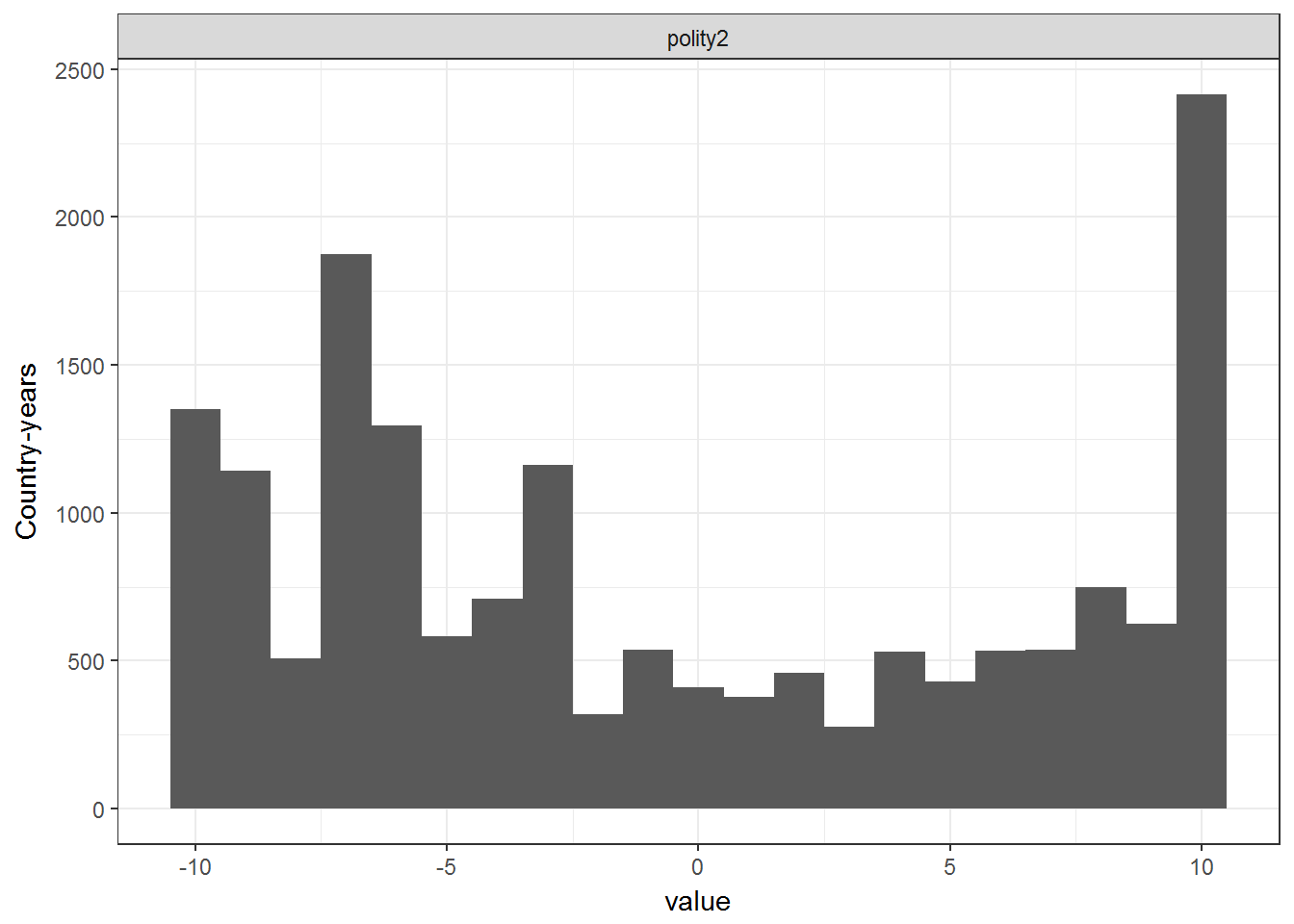
These are variables from the Polity IV dataset in country-year format, updated to 2014 (Marshall, Gurr, and Jaggers 2012).
The dataset from Coppedge and Reinicke 1991, revised in 2003-2006 with a new “contestation” measure.
data <- democracy_long %>% filter(variable == "polyarchy_reversed")
temporal_coverage(data) ## Joining, by = c("country_name", "year")
spatial_coverage(data)
data <- democracy_long %>% filter(variable %in% c("polyarchy_reversed","polyarchy_contestation"))
ggplot(data = data) +
geom_histogram(aes(x=value)) +
theme_bw() +
theme(legend.position = "bottom") +
labs(y = "Country-years") +
facet_wrap(~variable, ncol=2)## `stat_bin()` using `bins = 30`. Pick better value with `binwidth`.
kable(democracy %>%
filter(!is.na(polyarchy_reversed)) %>%
count(polyarchy_reversed,polyarchy_contestation),
caption = "Relationship between reversed polyarchy measure and polyarchy contestation measure")| polyarchy_reversed | polyarchy_contestation | n |
|---|---|---|
| 0 | 1 | 35 |
| 1 | 2 | 12 |
| 2 | 2 | 24 |
| 3 | 3 | 22 |
| 4 | 4 | 17 |
| 5 | 4 | 16 |
| 5 | 5 | 10 |
| 6 | 5 | 33 |
| 7 | 6 | 19 |
| 8 | 7 | 21 |
| 9 | 8 | 35 |
| 10 | 9 | 113 |
The dataset first described in Gasiorowski 1996, and updated and revised in Reich 2002.
A constructed regime variable from Przeworski 2013 (the Political Institutions and Political Events (PIPE) Data Set).
data <- democracy_long %>% filter(variable == "przeworski")
temporal_coverage(data) ## Joining, by = c("country_name", "year")
spatial_coverage(data)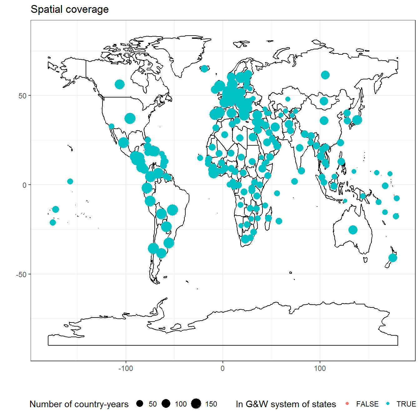
It is not clear that this index is correctly constructed, given the confusing documentation in the original dataset. Use with care.
ggplot(data = data) +
geom_histogram(aes(x=value)) +
theme_bw() +
theme(legend.position = "bottom") +
labs(y = "Country-years") +
facet_wrap(~variable, ncol=2)## `stat_bin()` using `bins = 30`. Pick better value with `binwidth`.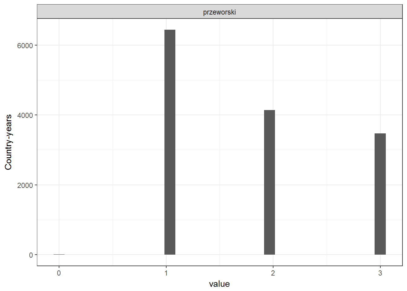
This uses a measure of democracy derived from the authoritarian regime dataset in Svolik 2012. The original data is extended to before 1946 using the information encoded in the o_startdate variable of the original dataset, which provides information for the start dates of some authoritarian regimes.
The dataset in Ulfelder 2012.
A measure of democracy from the regime type dataset described in Hsu 2008. This dataset identifies three types of democracies: “social democracies”, “conservative democracies”, and “one party democracies.” “One party democracies” are poorly documented, but seem to be equivalent to multiparty autocracies. utip_dichotomous_strict identifies as democracies only social or conservative democracies; utip_dichotomous also identifies as democracies those “one party democracies”; and utip_trichotomous assumes that “one party democracies” are hybrid regimes between democracy and non-democracy.
data <- democracy_long %>% filter(variable == "utip_dichotomous")
temporal_coverage(data) ## Joining, by = c("country_name", "year")
spatial_coverage(data)
data <- democracy_long %>% filter(variable %in% c("utip_dichotomous_strict","utip_dichotomous","utip_trichotomous"))
ggplot(data = data) +
geom_histogram(aes(x=value)) +
theme_bw() +
theme(legend.position = "bottom") +
labs(y = "Country-years") +
facet_wrap(~variable, ncol=2)## `stat_bin()` using `bins = 30`. Pick better value with `binwidth`.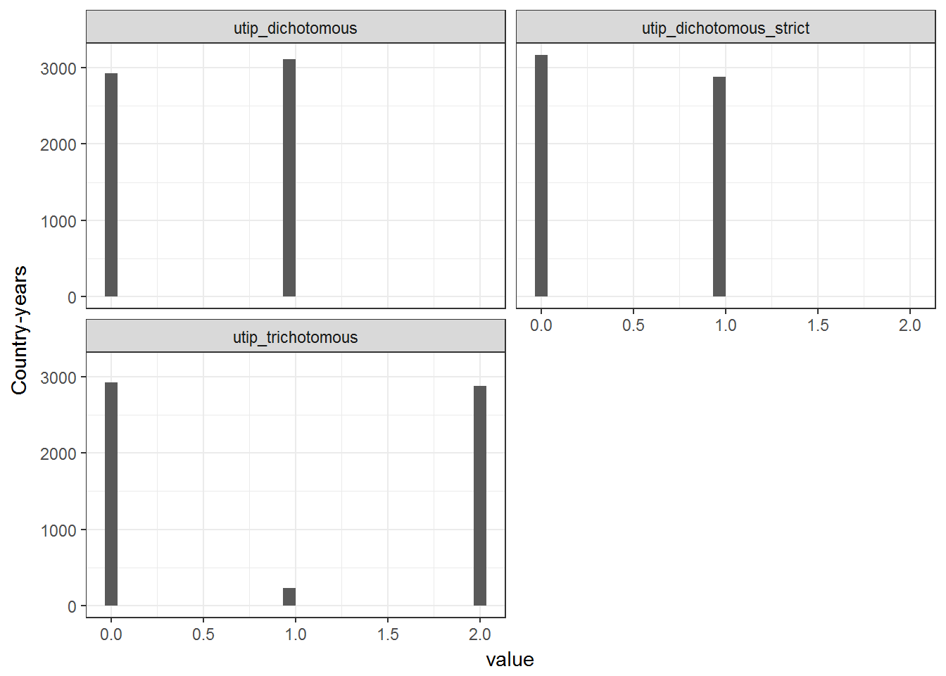
This is the dataset in Vanhanen 2012.
data <- democracy_long %>% filter(variable == "vanhanen_democratization")
temporal_coverage(data) ## Joining, by = c("country_name", "year")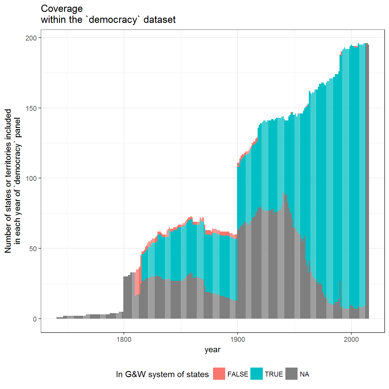
spatial_coverage(data)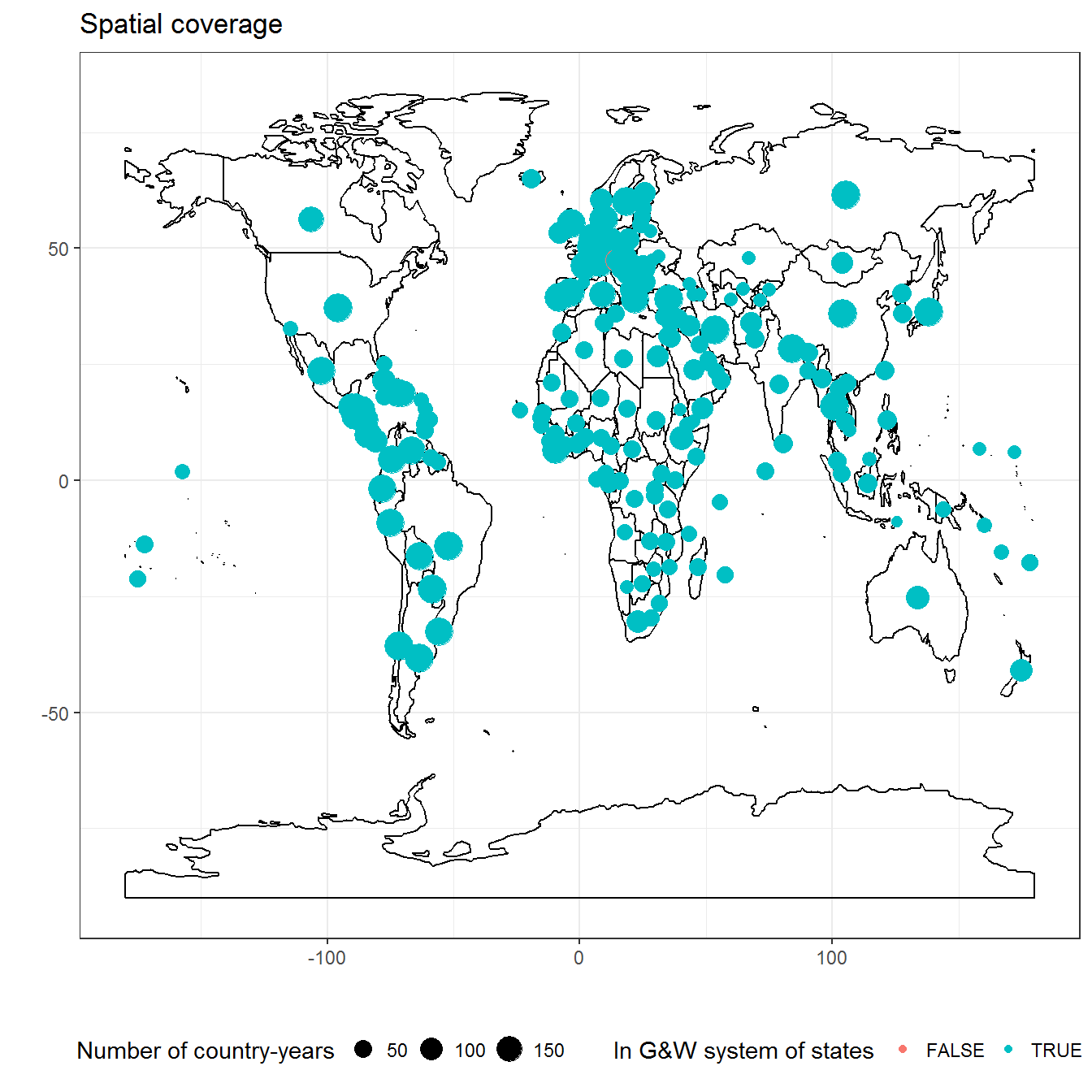
data <- democracy_long %>% filter(variable %in% c("vanhanen_democratization","vanhanen_participation","vanhanen_competition"))
ggplot(data = data) +
geom_histogram(aes(x=value)) +
theme_bw() +
theme(legend.position = "bottom") +
labs(y = "Country-years") +
facet_wrap(~variable, ncol=2)## `stat_bin()` using `bins = 30`. Pick better value with `binwidth`.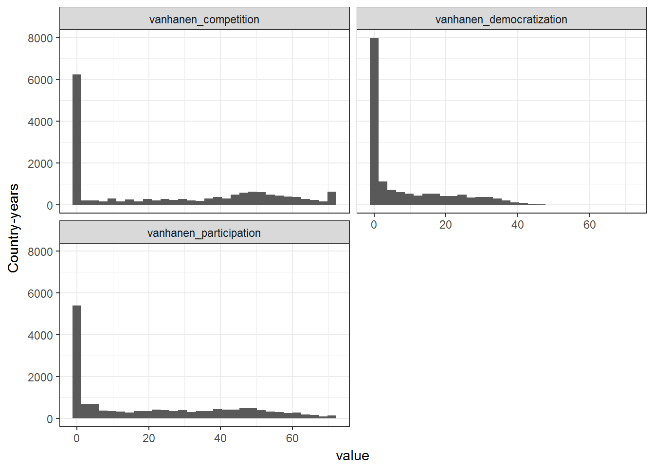
ggplot(data = data) +
  geom_density(aes(x=value)) +
  theme_bw() +
  theme(legend.position = "bottom") +
  labs(y = "Density") +
facet_wrap(~variable, ncol=2) 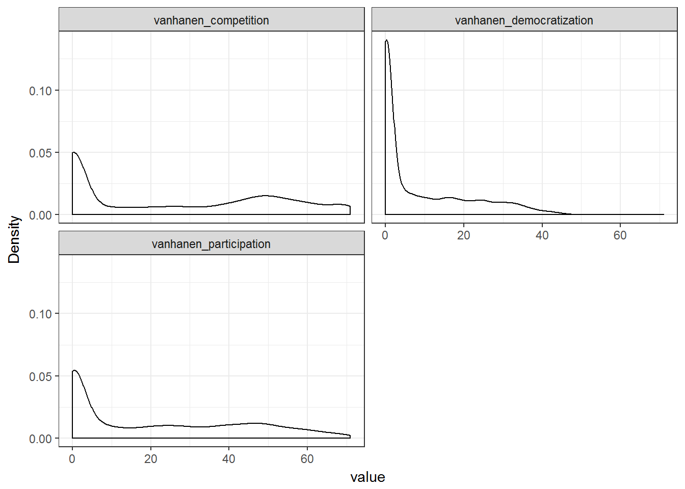
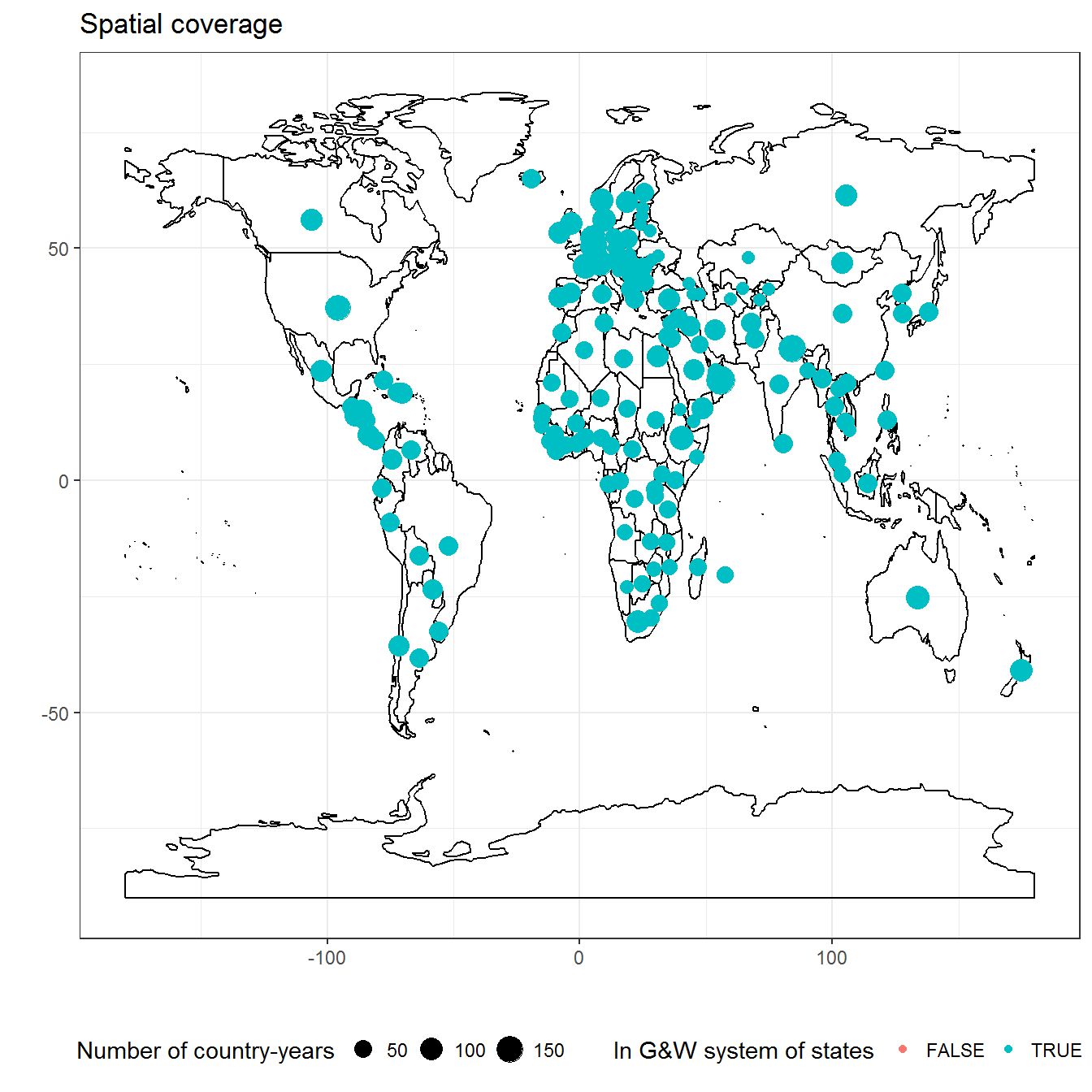
This is a selection of the major democracy indexes from version 6 of the V-Dem dataset (v2x* variables) (Coppedge et al. 2016).
Most of the not in-system country-years in the main dataset are from V-Dem.
data <- democracy_long %>% filter(variable == "v2x_polyarchy")
temporal_coverage(data) ## Joining, by = c("country_name", "year")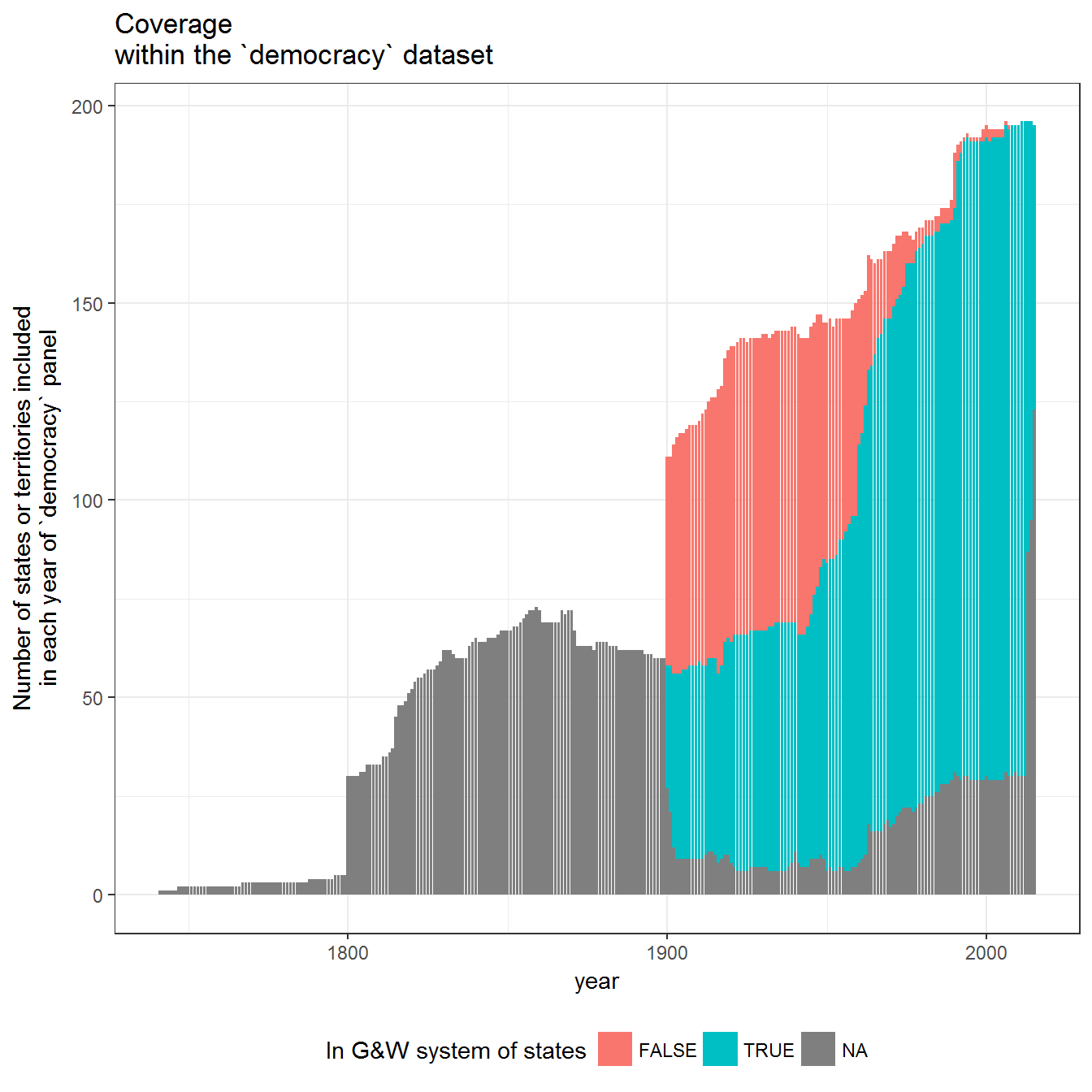
spatial_coverage(data)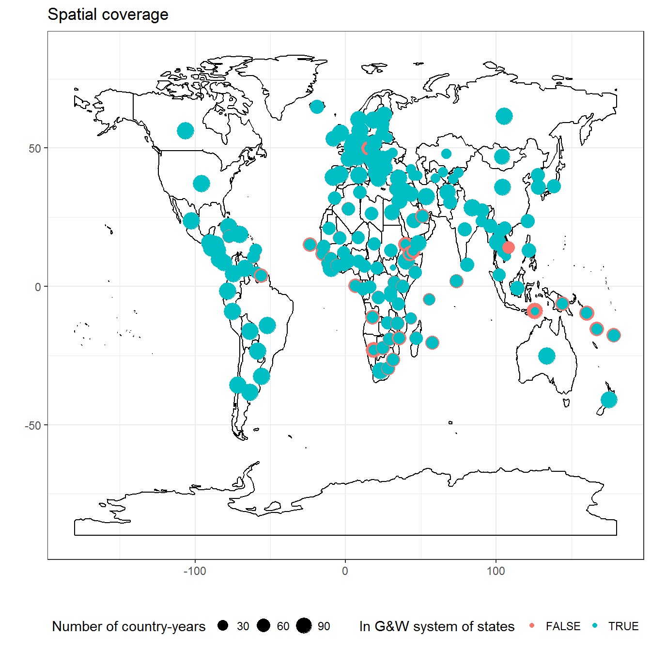
data <- democracy_long %>% filter(grepl("v2x",variable))
ggplot(data = data) +
  geom_histogram(aes(x=value)) +
  theme_bw() +
  theme(legend.position = "bottom") +
  labs(y = "Country-years") +
  facet_wrap(~variable, ncol=2)
## `stat_bin()` using `bins = 30`. Pick better value with `binwidth`.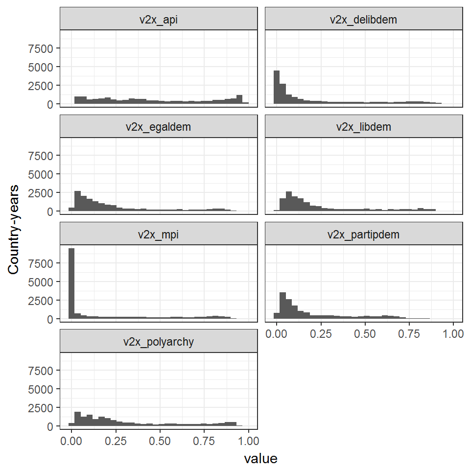
ggplot(data = data) +
  geom_density(aes(x=value)) +
  theme_bw() +
  theme(legend.position = "bottom") +
  labs(y = "Density") +
facet_wrap(~variable, ncol=2) 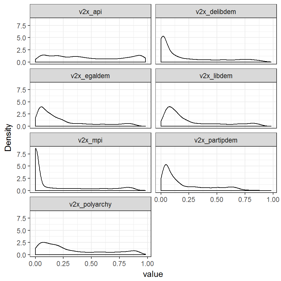
ggcorr(data = democracy %>% select(v2x_api:v2x_polyarchy), label=TRUE,label_round=3, hjust=1) + scale_fill_gradient2(midpoint = 0.7)## Scale for 'fill' is already present. Adding another scale for 'fill',
## which will replace the existing scale.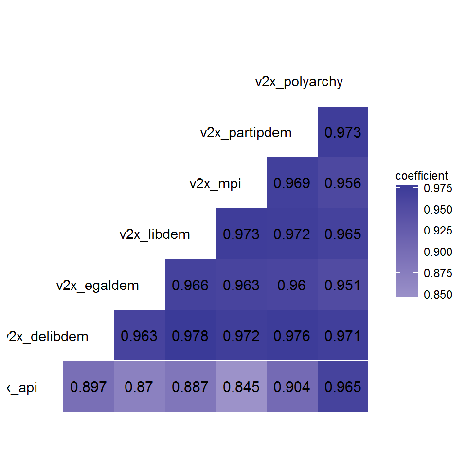
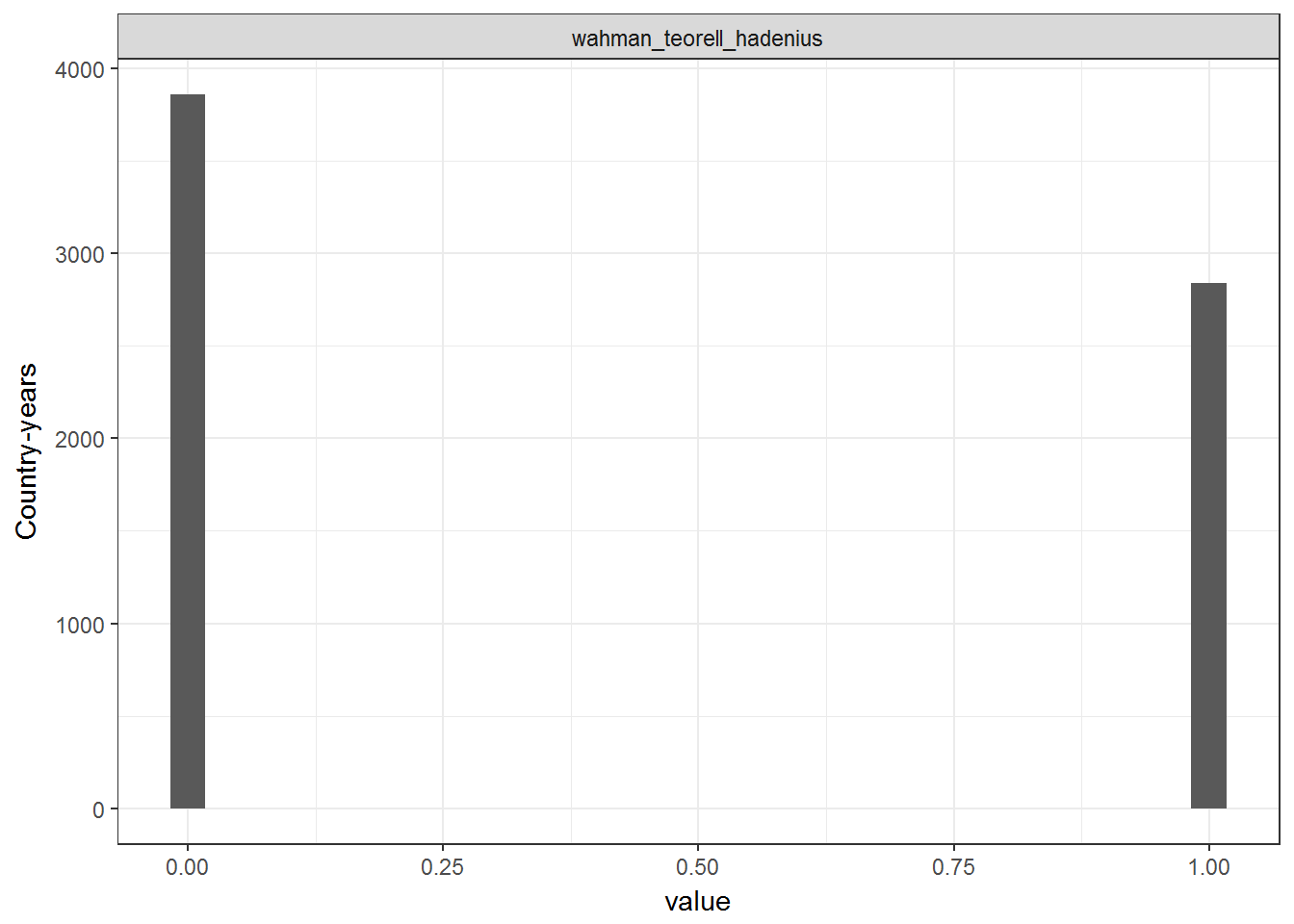
This is a measure of democracy from the authoritarian Regimes Data Set, version 5.0, by Hadenius, Teorell, & Wahman, described in Hadenius and Teorell 2007 and in Wahman, Teorell, Hadenius 2013.
count_sequence_breaks <- function(seq, seq_step = 1) {
  first_diff <- c(seq_step, diff(seq)) - seq_step
  periods <- cumsum(abs(first_diff))
  periods
}

kable(democracy %>%
        filter(GWn != cown | GWn != polity_ccode | cown != polity_ccode) %>%
        distinct(country_name,GWn,cown,polity_ccode,year) %>%
        arrange(country_name,GWn,cown,polity_ccode,year) %>%
        group_by(country_name,GWn,cown,polity_ccode) %>%
        mutate(period = count_sequence_breaks(year)) %>%
        group_by(period, add = TRUE) %>%
        summarise(min = min(year), max = max(year), n = n()),
caption = "Differences between Gleditsch and Ward codes, COW codes, and Polity codes")| country_name | GWn | cown | polity_ccode | period | min | max | n |
|---|---|---|---|---|---|---|---|
| Ethiopia | 530 | 530 | 529 | 0 | 1994 | 2015 | 22 |
| German Federal Republic | 260 | 255 | 255 | 0 | 1991 | 2015 | 25 |
| Italy/Sardinia | 325 | 325 | 324 | 0 | 1815 | 1860 | 46 |
| Kiribati | 970 | 946 | 946 | 0 | 1978 | 2015 | 38 |
| Kosovo | 347 | 347 | 341 | 0 | 1999 | 2015 | 17 |
| Montenegro | 341 | 341 | 348 | 0 | 1878 | 1917 | 40 |
| Montenegro | 341 | 341 | 348 | 81 | 1999 | 2015 | 17 |
| Nauru | 971 | 970 | 970 | 0 | 1968 | 2015 | 48 |
| Pakistan | 770 | 770 | 769 | 0 | 1947 | 1971 | 25 |
| Russia (Soviet Union) | 365 | 365 | 364 | 0 | 1923 | 1991 | 69 |
| Serbia | 340 | 345 | 342 | 0 | 1830 | 1920 | 91 |
| Serbia | 340 | 345 | 342 | 85 | 2006 | 2015 | 10 |
| South Sudan | 626 | 626 | 525 | 0 | 2011 | 2015 | 5 |
| Sudan | 625 | 625 | 626 | 0 | 1900 | 1947 | 48 |
| Sudan | 625 | 625 | 626 | 5 | 1953 | 1955 | 3 |
| Sudan | 625 | 625 | 626 | 60 | 2011 | 2015 | 5 |
| Tonga | 972 | 955 | 955 | 0 | 1963 | 2015 | 53 |
| Tuvalu | 973 | 947 | 947 | 0 | 1977 | 2015 | 39 |
| Vietnam (Annam/Cochin China/Tonkin) | 815 | 816 | 816 | 0 | 1800 | 1892 | 93 |
| Vietnam (Annam/Cochin China/Tonkin) | 815 | 816 | 816 | 9 | 1902 | 1948 | 47 |
| Vietnam, Democratic Republic of | 816 | 816 | 818 | 0 | 1945 | 1953 | 9 |
| Vietnam, Democratic Republic of | 816 | 816 | 818 | 22 | 1976 | 2015 | 40 |
| Yemen (Arab Republic of Yemen) | 678 | 679 | 679 | 0 | 1990 | 2015 | 26 |
| Yugoslavia | 345 | 345 | 347 | 0 | 1913 | 1920 | 8 |
| Yugoslavia | 345 | 345 | 347 | 70 | 1991 | 2006 | 16 |
There are a few country-years that are in the CoW state system but are not included in this dataset:
COW_system <- read.csv("http://www.correlatesofwar.org/data-sets/state-system-membership/system2011/at_download/file")

COW_system <- COW_system %>% rename(cown = ccode)

kable(anti_join(COW_system,democracy))
## Joining, by = c("cown", "year")| stateabb | cown | year | version |
|---|---|---|---|
| YAR | 678 | 1990 | 2011 |
| ZAN | 511 | 1964 | 2011 |
| SIC | 329 | 1861 | 2011 |
| GMY | 255 | 1990 | 2011 |
| AUH | 300 | 1918 | 2011 |
| TUN | 616 | 1881 | 2011 |
| EGY | 651 | 1882 | 2011 |
Germany in 1990 appears with the GWn code 260 for 1990, since Gleditsch and Ward treats it as a continuation of the Federal Republic; similarly, the Yemen Arab Republic appears with the GWn code 678 for 1990, since Gleditsch and Ward treat is a continuation of the previous state, while CoW considers it a new state (code 679). The rest - Zanzibar 1964, Sicily (Kingdom of the Two Sicilies) 1861, Austria-Hungary 1918, Tunisia 1881, and Egypt 1882 have no data for the democracy measures. These cases also represent years where these countries lost their independence or disappeared.
It is also worth noting that, though there are no duplicate country-years wehn grouping by country_name or GWn or polity_ccode, when grouping by cown, there are a few duplicate observations:
kable(democracy %>%
        group_by(country_name,year) %>%
        filter(n() > 1) %>%
        group_by(country_name) %>%
summarise(countries = paste(unique(country_name),collapse = ", "), min(year), max(year)))| country_name | countries | min(year) | max(year) |
|---|
kable(democracy %>%
        group_by(GWn,year) %>%
        filter(n() > 1) %>%
        group_by(GWn) %>%
summarise(countries = paste(unique(country_name),collapse = ", "), min(year), max(year)))| GWn | countries | min(year) | max(year) |
|---|
kable(democracy %>%
        group_by(polity_ccode,year) %>%
        filter(n() > 1) %>%
        group_by(polity_ccode) %>%
summarise(countries = paste(unique(country_name),collapse = ", "), min(year), max(year)))| polity_ccode | countries | min(year) | max(year) |
|---|
kable(democracy %>%
        group_by(cown,year) %>%
        filter(n() > 1) %>%
        group_by(cown) %>%
summarise(countries = paste(unique(country_name),collapse = ", "), min(year), max(year)))| cown | countries | min(year) | max(year) |
|---|---|---|---|
| 345 | Serbia, Yugoslavia | 1913 | 2006 |
| 816 | Vietnam (Annam/Cochin China/Tonkin), Vietnam, Democratic Republic of | 1945 | 1948 |
Arat, Zehra F. 1991. Democracy and human rights in developing countries. Boulder: Lynne Rienner Publishers.
Bernhard, Michael Timothy Nordstrom, and Christopher Reenock, “Economic Performance, Institutional Intermediation and Democratic Breakdown,” Journal of Politics 63:3 (2001), pp. 775-803. Data and coding description available at http://users.clas.ufl.edu/bernhard/content/data/data.htm
Boix, Carles, Michael Miller, and Sebastian Rosato. 2012. A Complete Data Set of Political Regimes, 1800-2007. Comparative Political Studies 46 (12): 1523-1554. Original data available at https://sites.google.com/site/mkmtwo/democracy-v2.0.dta?attredirects=0
Bollen, Kenneth A. 2001. “Cross-National Indicators of Liberal Democracy, 1950-1990.” 2nd ICPSR version. Chapel Hill, NC: University of North Carolina, 1998. Ann Arbor, MI: Inter-university Consortium for Political and Social Research, 2001. Original data available at http://webapp.icpsr.umich.edu/cocoon/ICPSR-STUDY/02532.xml.
Bowman, Kirk, Fabrice Lehoucq, and James Mahoney. 2005. Measuring Political Democracy: Case Expertise, Data Adequacy, and Central America. Comparative Political Studies 38 (8): 939-970. http://cps.sagepub.com/content/38/8/939. Data available at http://www.blmdemocracy.gatech.edu/.
Cheibub, Jose Antonio, Jennifer Gandhi, and James Raymond Vreeland. 2010. “Democracy and Dictatorship Revisited.” Public Choice. 143(1):67-101. Original data available at https://sites.google.com/site/joseantoniocheibub/datasets/democracy-and-dictatorship-revisited.
Coppedge, Michael, John Gerring, Staffan I. Lindberg, Svend-Erik Skaaning, and Jan Teorell, with David Altman, Michael Bernhard, M. Steven Fish, Adam Glynn, Allen Hicken, Carl Henrik Knutsen, Kelly McMann, Pamela Paxton, Daniel Pemstein, Jeffrey Staton, Brigitte Zimmerman, Frida Andersson, Valeriya Mechkova, Farhad Miri. 2015. V-Dem Codebook v5. Varieties of Democracy (V-Dem) Project. Original data available at https://v-dem.net/en/data/.
Coppedge, Michael and Wolfgang H. Reinicke. 1991. Measuring Polyarchy. In On Measuring Democracy: Its Consequences and Concomitants, ed. Alex Inkeles. New Brunswuck, NJ: Transaction pp. 47-68.
Doorenspleet, Renske. 2000. Reassessing the Three Waves of Democratization. World Politics 52 (03): 384-406. DOI: 10.1017/S0043887100016580. http://dx.doi.org/10.1017/S0043887100016580.
Economist Intelligence Unit. 2012. Democracy Index 2012: Democracy at a Standstill.
Freedom House. 2015. “Freedom in the World.” Original data available at http://www.freedomhouse.org.
Gasiorowski, Mark J. 1996. “An Overview of the Political Regime Change Dataset.” Comparative Political Studies 29(4):469-483.
Geddes, Barbara, Joseph Wright, and Erica Frantz. 2014. Autocratic Breakdown and Regime Transitions: A New Data Set. Perspectives on Politics 12 (1): 313-331. Original data available at http://dictators.la.psu.edu/.
Gleditsch, Kristian S. & Michael D. Ward. 1999. “Interstate System Membership: A Revised List of the Independent States since 1816.” International Interactions 25: 393-413. The list can be found at http://privatewww.essex.ac.uk/~ksg/statelist.html
Goldstone, Jack, Robert Bates, David Epstein, Ted Gurr, Michael Lustik, Monty Marshall, Jay Ulfelder, and Mark Woodward. 2010. A Global Model for Forecasting Political Instability. American Journal of Political Science 54 (1): 190-208. DOI:10.1111/j.1540-5907.2009.00426.x
Hadenius, Axel. 1992. Democracy and Development. Cambridge: Cambridge University Press.
Hadenius, Axel & Jan Teorell. 2007. “Pathways from Authoritarianism”, Journal of Democracy 18(1): 143-156.
Hsu, Sara “The Effect of Political Regimes on Inequality, 1963-2002,” UTIP Working Paper No. 53 (2008), http://utip.gov.utexas.edu/papers/utip_53.pdf. Data available for download at http://utip.gov.utexas.edu/data/.
Kailitz, Steffen. 2013. Classifying political regimes revisited: legitimation and durability. Democratization 20 (1): 39-60. Original data available at http://dx.doi.org/10.1080/13510347.2013.738861.
Mainwaring, Scott, Daniel Brinks, and Anibal Perez Linan. 2008. “Political Regimes in Latin America, 1900-2007.” Original data available from http://kellogg.nd.edu/scottmainwaring/Political_Regimes.pdf.
Magaloni, Beatriz, Jonathan Chu, and Eric Min. 2013. Autocracies of the World, 1950-2012 (Version 1.0). Dataset, Stanford University. Original data and codebook available at http://cddrl.fsi.stanford.edu/research/autocracies_of_the_world_dataset/
Marshall, Monty G., Ted Robert Gurr, and Keith Jaggers. 2012. “Polity IV: Political Regime Characteristics and Transitions, 1800-2012.” Updated to 2015. Original data available from http://www.systemicpeace.org/polity/polity4.htm.
Moon, Bruce E., Jennifer Harvey Birdsall, Sylvia Ceisluk, Lauren M. Garlett, Joshua J. Hermias, Elizabeth Mendenhall, Patrick D. Schmid, and Wai Hong Wong (2006) “Voting Counts: Participation in the Measurement of Democracy” Studies in Comparative International Development 42, 2 (Summer, 2006). The complete dataset is available here: http://www.lehigh.edu/~bm05/democracy/Obtain_data.htm.
Munck, Gerardo L. 2009. Measuring Democracy: A Bridge Between Scholarship and Politics. Baltimore: Johns Hopkins University Press.
Pemstein, Daniel, Stephen Meserve, and James Melton. 2010. Democratic Compromise: A Latent Variable Analysis of Ten Measures of Regime Type. Political Analysis 18 (4): 426-449.
Pemstein, Daniel, Stephen A. Meserve, and James Melton. 2013. “Replication data for: Democratic Compromise: A Latent Variable Analysis of Ten Measures of Regime Type.” In: Harvard Dataverse. http://hdl.handle.net/1902.1/PMM
Przeworski, Adam et al. 2013. Political Institutions and Political Events (PIPE) Data Set. Department of Politics, New York University. https://sites.google.com/a/nyu.edu/adam-przeworski/home/data
Reich, G. 2002. Categorizing Political Regimes: New Data for Old Problems. Democratization 9 (4): 1-24. http://www.tandfonline.com/doi/pdf/10.1080/714000289.
Skaaning, Svend-Erik, John Gerring, and Henrikas Bartusevicius. 2015. A Lexical Index of Electoral Democracy. Comparative Political Studies 48 (12): 1491-1525. Original data available from http://thedata.harvard.edu/dvn/dv/skaaning.
Svolik, Milan. 2012. The Politics of Authoritarian Rule. Cambridge and New York: Cambridge University Press. Original data available from http://campuspress.yale.edu/svolik/the-politics-of-authoritarian-rule/.
Taylor, Sean J. and Ulfelder, Jay, A Measurement Error Model of Dichotomous Democracy Status (May 20, 2015). Available at SSRN: http://ssrn.com/abstract=2726962 or http://dx.doi.org/10.2139/ssrn.2726962
Ulfelder, Jay. 2012. “Democracy/Autocracy Data Set.” In: Harvard Dataverse. http://hdl.handle.net/1902.1/18836.
Vanhanen, Tatu. 2012. “FSD1289 Measures of Democracy 1810-2012.” Original data available from http://www.fsd.uta.fi/english/data/catalogue/FSD1289/meF1289e.html
Wahman, Michael, Jan Teorell, and Axel Hadenius. 2013. Authoritarian regime types revisited: updated data in comparative perspective. Contemporary Politics 19 (1): 19-34.